设计自适应实验来研究工作记忆
在大多数机器学习中,我们从数据开始,然后学习模型。在其他情况下,我们也可以参与数据生成过程。这给了我们一个令人兴奋的机会:我们可以尝试获取有助于模型更有效学习的数据。这个过程被称为最优实验设计 (OED),Pyro 通过 pyro.contrib.oed 模块支持选择最优设计。
使用 OED 时,数据生成和建模过程如下
写下一个贝叶斯模型,其中包含一个设计参数、一个未知隐变量和一个可观测变量。
选择最优设计(稍后详述)。
收集数据并拟合模型,例如使用
SVI。
我们还可以进行多轮或多次实验迭代。这样做时,我们将从步骤 3 中学到的模型用作下一轮步骤 1 中的先验。这种方法特别有用,因为它允许我们根据已经学到的东西来设计下一个实验:实验是自适应的。
在本教程中,我们将通过一个具体的例子来展示多轮 OED 的整个过程。我们将展示如何设计自适应实验来学习参与者的工作记忆容量。我们将要自适应的设计是要求参与者记住的数字序列的长度。让我们深入了解完整的细节。
实验设置
假设你,作为参与者,被展示一个数字序列
然后将其隐藏。你必须凭记忆准确地重现这个序列。在下一轮中,序列的长度可能会不同
你能记住的最长序列就是你的工作记忆容量。在本教程中,我们建立一个工作记忆的贝叶斯模型,并用它来运行一系列自适应实验,从而非常快速地学习某人的工作记忆容量。
工作记忆模型
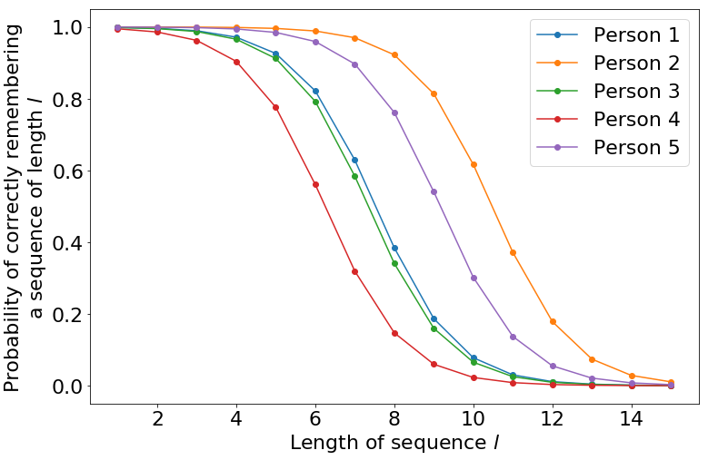
我们为上述数字实验的单轮建立的模型包含三个组成部分:参与者需要记住的序列长度 \(l\),参与者的真实工作记忆容量 \(\theta\),以及实验结果 \(y\),表示他们是否成功记住序列(\(y=1\))或未能记住(\(y=0\))。我们根据(臭名昭著的)“神奇的数字七,加减二”[1]选择工作记忆容量的先验。
注意:\(\theta\) 实际上代表了参与者正确记住序列的概率为 50/50 的那个点。
[2]:
import torch

import pyro
import pyro.distributions as dist


sensitivity = 1.0
prior_mean = torch.tensor(7.0)
prior_sd = torch.tensor(2.0)


def model(l):
    # Dimension -1 of `l` represents the number of rounds
    # Other dimensions are batch dimensions: we indicate this with a plate_stack
    with pyro.plate_stack("plate", l.shape[:-1]):
        theta = pyro.sample("theta", dist.Normal(prior_mean, prior_sd))
        # Share theta across the number of rounds of the experiment
        # This represents repeatedly testing the same participant
        theta = theta.unsqueeze(-1)
        # This define a *logistic regression* model for y
        logit_p = sensitivity * (theta - l)
        # The event shape represents responses from the same participant
        y = pyro.sample("y", dist.Bernoulli(logits=logit_p).to_event(1))
        return y
成功记住序列的概率如下所示,针对 \(\theta\) 的五个随机样本进行了绘制。
[4]:
import matplotlib
import matplotlib.pyplot as plt

matplotlib.rcParams.update({'font.size': 22})

# We sample five times from the prior
theta = (prior_mean + prior_sd * torch.randn((5,1)))
l = torch.arange(1, 16, dtype=torch.float)
# This is the same as using 'logits=' in the prior above
prob = torch.sigmoid(sensitivity * (theta - l))

plt.figure(figsize=(12, 8))
for curve in torch.unbind(prob, 0):
    plt.plot(l.numpy(), curve.numpy(), marker='o')
plt.xlabel("Length of sequence $l$")
plt.ylabel("Probability of correctly remembering\na sequence of length $l$")
plt.legend(["Person {}".format(i+1) for i in range(5)])
plt.show()
模型推断
有了这个模型,我们快速演示一下 Pyro 中对这个模型的变分推断。我们定义一个 Normal 引导(guide)用于变分推断。
[5]:
from torch.distributions.constraints import positive

def guide(l):
    # The guide is initialised at the prior
    posterior_mean = pyro.param("posterior_mean", prior_mean.clone())
    posterior_sd = pyro.param("posterior_sd", prior_sd.clone(), constraint=positive)
    pyro.sample("theta", dist.Normal(posterior_mean, posterior_sd))
最后,我们指定以下数据:参与者被展示了长度为 5、7 和 9 的序列。他们正确记住了前两个,但没有记住第三个。
[6]:
l_data = torch.tensor([5., 7., 9.])
y_data = torch.tensor([1., 1., 0.])
现在我们可以对模型运行 SVI。
[7]:
from pyro.infer import SVI, Trace_ELBO
from pyro.optim import Adam

conditioned_model = pyro.condition(model, {"y": y_data})
svi = SVI(conditioned_model,
          guide,
          Adam({"lr": .001}),
          loss=Trace_ELBO(),
          num_samples=100)
pyro.clear_param_store()
num_iters = 5000
for i in range(num_iters):
    elbo = svi.step(l_data)
    if i % 500 == 0:
        print("Neg ELBO:", elbo)
Neg ELBO: 1.6167092323303223
Neg ELBO: 3.706324815750122
Neg ELBO: 0.9958380460739136
Neg ELBO: 1.0630500316619873
Neg ELBO: 1.1738307476043701
Neg ELBO: 1.6654635667800903
Neg ELBO: 1.296904444694519
Neg ELBO: 1.305729627609253
Neg ELBO: 1.2626266479492188
Neg ELBO: 1.3095542192459106
[9]:
print("Prior:     N({:.3f}, {:.3f})".format(prior_mean, prior_sd))
print("Posterior: N({:.3f}, {:.3f})".format(pyro.param("posterior_mean"),
                                            pyro.param("posterior_sd")))
Prior:     N(7.000, 2.000)
Posterior: N(7.749, 1.282)
在我们的后验分布下,我们可以看到我们对参与者工作记忆容量有了更新的估计,并且我们的不确定性现在降低了。
贝叶斯最优实验设计
到目前为止都很标准。在前面的例子中,长度 l_data 的选择并没有经过深思熟虑。幸运的是,在这种情况下,可以使用更复杂的策略来选择序列长度,以充分利用我们提出的每个问题。
我们使用贝叶斯最优实验设计 (BOED) 来做到这一点。在 BOED 中,我们感兴趣的是设计能够最大化信息增益的实验,其正式定义为
其中 \(KL\) 代表 Kullback-Leiber 散度。
换句话说,信息增益是后验分布与先验分布之间的 KL 散度。因此,它代表了我们通过运行长度为 \(l\) 的实验并获得结果 \(y\) 来“移动”后验分布的距离。
不幸的是,在实际运行实验之前,我们无法知道 \(y\)。因此,我们基于预期信息增益 [2] 来选择 \(l\)
由于它包含后验密度 \(p(y|\theta,l)\),EIG 并不直接可计算。然而,我们可以利用以下 EIG 的变分估计器 [3]
Pyro 中的最优实验设计
幸运的是,Pyro 提供了估算 EIG 的现成工具。我们只需在上面的公式中定义“边际引导”(marginal guide)\(q(y|l)\)。
[10]:
def marginal_guide(design, observation_labels, target_labels):
    # This shape allows us to learn a different parameter for each candidate design l
    q_logit = pyro.param("q_logit", torch.zeros(design.shape[-2:]))
    pyro.sample("y", dist.Bernoulli(logits=q_logit).to_event(1))
这不像在 Pyro 中通常遇到并用于 SVI 的那些引导用于推断。相反,这种引导只采样观测到的采样点:在本例中是 "y"。这是有道理的,因为传统引导近似后验分布 \(p(\theta|y, l)\),而我们的引导近似边际分布 \(p(y|l)\)。
[11]:
from pyro.contrib.oed.eig import marginal_eig

# The shape of `candidate_designs` is (number designs, 1)
# This represents a batch of candidate designs, each design is for one round of experiment
candidate_designs = torch.arange(1, 15, dtype=torch.float).unsqueeze(-1)
pyro.clear_param_store()
num_steps, start_lr, end_lr = 1000, 0.1, 0.001
optimizer = pyro.optim.ExponentialLR({'optimizer': torch.optim.Adam,
                                      'optim_args': {'lr': start_lr},
                                      'gamma': (end_lr / start_lr) ** (1 / num_steps)})

eig = marginal_eig(model,
                   candidate_designs,       # design, or in this case, tensor of possible designs
                   "y",                     # site label of observations, could be a list
                   "theta",                 # site label of 'targets' (latent variables), could also be list
                   num_samples=100,         # number of samples to draw per step in the expectation
                   num_steps=num_steps,     # number of gradient steps
                   guide=marginal_guide,    # guide q(y)
                   optim=optimizer,         # optimizer with learning rate decay
                   final_num_samples=10000  # at the last step, we draw more samples
                                            # for a more accurate EIG estimate
                  )
我们可以将找到的 EIG 估计值可视化。
[12]:
plt.figure(figsize=(10,5))
matplotlib.rcParams.update({'font.size': 22})
plt.plot(candidate_designs.numpy(), eig.detach().numpy(), marker='o', linewidth=2)
plt.xlabel("$l$")
plt.ylabel("EIG($l$)")
plt.show()
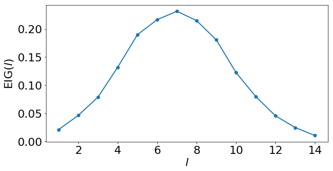
[13]:
best_l = 1 + torch.argmax(eig)
print("Optimal design:", best_l.item())
Optimal design: 7
这告诉我们第一轮实验应该使用长度为 7 的序列。请注意,虽然我们可能凭直觉猜到这个最优设计,但同样的框架同样适用于更复杂的模型和实验,在这些场景中凭直觉找到最优设计更具挑战性。
作为训练的附带结果,我们的边际引导 \(q(y|l)\) 近似地学习了边际分布 \(p(y|l)\)。
[14]:
q_prob = torch.sigmoid(pyro.param("q_logit"))
print("   l | q(y = 1 | l)")
for (l, q) in zip(candidate_designs, q_prob):
    print("{:>4} | {}".format(int(l.item()), q.item()))
   l | q(y = 1 | l)
   1 | 0.9849993586540222
   2 | 0.9676634669303894
   3 | 0.9329487681388855
   4 | 0.871809720993042
   5 | 0.7761920690536499
   6 | 0.6436398029327393
   7 | 0.4999988079071045
   8 | 0.34875917434692383
   9 | 0.22899287939071655
  10 | 0.13036076724529266
  11 | 0.06722454726696014
  12 | 0.03191758319735527
  13 | 0.015132307074964046
  14 | 0.00795808993279934
这个拟合张量的元素代表了对于 candidate_designs 中每个可能的序列长度 \(l\) 对应的 \(y\) 的边际分布。我们已经对未知变量 \(\theta\) 进行了边缘化,因此这个拟合张量显示的是“平均”参与者的概率。
自适应实验
现在我们有了构建自适应实验来研究工作记忆的要素。我们重复以下步骤
使用 EIG 找到最优序列长度 \(l\)
使用长度为 \(l\) 的序列进行测试
用新数据更新后验分布
在第一次迭代中,步骤 1 使用上述先验。然而,对于后续迭代,我们使用基于所有现有数据的后验。
在本 notebook 中,“实验”使用以下合成器进行
[15]:
def synthetic_person(l):
    # The synthetic person can remember any sequence shorter than 6
    # They cannot remember any sequence of length 6 or above
    # (There is no randomness in their responses)
    y = (l < 6.).float()
    return y
以下代码允许我们在收集更多数据时更新模型。
[16]:
def make_model(mean, sd):
    def model(l):
        # Dimension -1 of `l` represents the number of rounds
        # Other dimensions are batch dimensions: we indicate this with a plate_stack
        with pyro.plate_stack("plate", l.shape[:-1]):
            theta = pyro.sample("theta", dist.Normal(mean, sd))
            # Share theta across the number of rounds of the experiment
            # This represents repeatedly testing the same participant
            theta = theta.unsqueeze(-1)
            # This define a *logistic regression* model for y
            logit_p = sensitivity * (theta - l)
            # The event shape represents responses from the same participant
            y = pyro.sample("y", dist.Bernoulli(logits=logit_p).to_event(1))
            return y
    return model
现在我们准备好了,可以运行一个使用自适应设计的 10 步实验。
[17]:
ys = torch.tensor([])
ls = torch.tensor([])
history = [(prior_mean, prior_sd)]
pyro.clear_param_store()
current_model = make_model(prior_mean, prior_sd)

for experiment in range(10):
    print("Round", experiment + 1)

    # Step 1: compute the optimal length
    optimizer = pyro.optim.ExponentialLR({'optimizer': torch.optim.Adam,
                                          'optim_args': {'lr': start_lr},
                                          'gamma': (end_lr / start_lr) ** (1 / num_steps)})
    eig = marginal_eig(current_model, candidate_designs, "y", "theta", num_samples=100,
                       num_steps=num_steps, guide=marginal_guide, optim=optimizer,
                       final_num_samples=10000)
    best_l = 1 + torch.argmax(eig).float().detach()

    # Step 2: run the experiment, here using the synthetic person
    print("Asking the participant to remember a sequence of length", int(best_l.item()))
    y = synthetic_person(best_l)
    if y:
        print("Participant remembered correctly")
    else:
        print("Participant could not remember the sequence")
    # Store the sequence length and outcome
    ls = torch.cat([ls, best_l.expand(1)], dim=0)
    ys = torch.cat([ys, y.expand(1)])

    # Step 3: learn the posterior using all data seen so far
    conditioned_model = pyro.condition(model, {"y": ys})
    svi = SVI(conditioned_model,
              guide,
              Adam({"lr": .005}),
              loss=Trace_ELBO(),
              num_samples=100)
    num_iters = 2000
    for i in range(num_iters):
        elbo = svi.step(ls)

    history.append((pyro.param("posterior_mean").detach().clone().numpy(),
                    pyro.param("posterior_sd").detach().clone().numpy()))
    current_model = make_model(pyro.param("posterior_mean").detach().clone(),
                               pyro.param("posterior_sd").detach().clone())
    print("Estimate of \u03b8: {:.3f} \u00b1 {:.3f}\n".format(*history[-1]))
Round 1
Asking the participant to remember a sequence of length 7
Participant could not remember the sequence
Estimate of θ: 5.788 ± 1.636

Round 2
Asking the participant to remember a sequence of length 6
Participant could not remember the sequence
Estimate of θ: 4.943 ± 1.252

Round 3
Asking the participant to remember a sequence of length 5
Participant remembered correctly
Estimate of θ: 5.731 ± 1.043

Round 4
Asking the participant to remember a sequence of length 6
Participant could not remember the sequence
Estimate of θ: 5.261 ± 0.928

Round 5
Asking the participant to remember a sequence of length 5
Participant remembered correctly
Estimate of θ: 5.615 ± 0.859

Round 6
Asking the participant to remember a sequence of length 6
Participant could not remember the sequence
Estimate of θ: 5.423 ± 0.888

Round 7
Asking the participant to remember a sequence of length 6
Participant could not remember the sequence
Estimate of θ: 5.092 ± 0.763

Round 8
Asking the participant to remember a sequence of length 5
Participant remembered correctly
Estimate of θ: 5.371 ± 0.717

Round 9
Asking the participant to remember a sequence of length 5
Participant remembered correctly
Estimate of θ: 5.597 ± 0.720

Round 10
Asking the participant to remember a sequence of length 6
Participant could not remember the sequence
Estimate of θ: 5.434 ± 0.640
现在我们可视化 \((\theta)\) 的后验分布演变
[19]:
import numpy as np
from scipy.stats import norm
import matplotlib.colors as colors
import matplotlib.cm as cmx


matplotlib.rcParams.update({'font.size': 22})
cmap = plt.get_cmap('winter')
cNorm  = colors.Normalize(vmin=0, vmax=len(history)-1)
scalarMap = cmx.ScalarMappable(norm=cNorm, cmap=cmap)
plt.figure(figsize=(12, 6))
x = np.linspace(0, 14, 100)
for idx, (mean, sd) in enumerate(history):
    color = scalarMap.to_rgba(idx)
    y = norm.pdf(x, mean, sd)
    plt.plot(x, y, color=color)
    plt.xlabel("$\\theta$")
    plt.ylabel("p.d.f.")
plt.show()
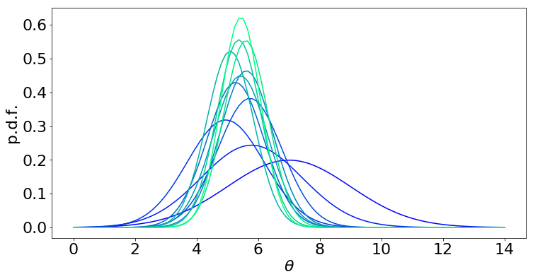
(蓝色 = 先验,浅绿色 = 10 步后验)
相比之下,假设我们使用一种简单的设计:尝试长度为 1, 2, …, 10 的序列。
[20]:
pyro.clear_param_store()
ls = torch.arange(1, 11, dtype=torch.float)
ys = synthetic_person(ls)
conditioned_model = pyro.condition(model, {"y": ys})
svi = SVI(conditioned_model,
          guide,
          Adam({"lr": .005}),
          loss=Trace_ELBO(),
          num_samples=100)
num_iters = 2000
for i in range(num_iters):
    elbo = svi.step(ls)
[22]:
plt.figure(figsize=(12,6))
matplotlib.rcParams.update({'font.size': 22})
y1 = norm.pdf(x, pyro.param("posterior_mean").detach().numpy(),
              pyro.param("posterior_sd").detach().numpy())
y2 = norm.pdf(x, history[-1][0], history[-1][1])
plt.plot(x, y1)
plt.plot(x, y2)
plt.legend(["Simple design", "Optimal design"])
plt.xlabel("$\\theta$")
plt.ylabel("p.d.f.")
plt.show()
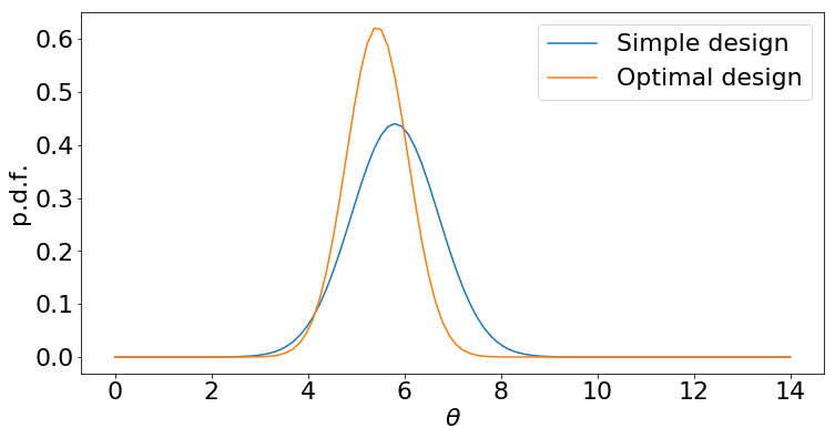
尽管两种设计策略都能提供数据,但最优策略最终得到的后验分布更尖锐:这意味着我们对最终答案更有信心,或者可以更早停止实验。
扩展
在本教程中,我们使用变分推断来拟合 \(\theta\) 的近似后验。这可以用其他后验推断策略代替,例如哈密顿蒙特卡洛(Hamiltonian Monte Carlo)。
本教程中的模型非常简单,可以通过多种方式进行扩展。例如,除了衡量参与者是否记住了序列,我们还可能收集其他信息。我们可以建立一个模型来预测犯错的数量(例如,正确序列与参与者回应之间的编辑距离),或者联合建模正确性和响应时间。这里有一个示例模型,我们使用 LogNormal 分布来模拟响应时间,如 [4] 所示。
[18]:
time_intercept = 0.5
time_scale = 0.5

def model(l):
    theta = pyro.sample("theta", dist.Normal(prior_mean, prior_sd))
    logit_p = sensitivity * (theta - l)
    correct = pyro.sample("correct", dist.Bernoulli(logits=logit_p))
    mean_log_time = time_intercept + time_scale * (theta - l)
    time = pyro.sample("time", dist.LogNormal(mean_log_time, 1.0))
    return correct, time
仍然可以使用 marginal_eig 计算 EIG。我们会将 "y" 替换为 ["correct", "time"],并且边际引导现在将对 "correct" 和 "time" 这两个点的联合分布进行建模。
我们的模型还做了一些假设,我们可以选择放宽这些假设。例如,我们假设所有相同长度的序列都同样容易记住。我们还将 sensitivity 固定为一个已知常数:我们可能需要学习这个值。我们还可以考虑在两个层面上进行学习:学习用于群体趋势的全局变量,以及用于个体效应的局部变量。当前模型只是一个针对个体的模型。在这些场景下,EIG 仍然可以作为选择最优设计的手段。
参考文献
[1] Miller, G.A., 1956. The magical number seven, plus or minus two: Some limits on our capacity for processing information. Psychological review, 63(2), p.81.
[2] Chaloner, K. and Verdinelli, I., 1995. Bayesian experimental design: A review. Statistical Science, pp.273-304.
[3] Foster, A., Jankowiak, M., Bingham, E., Horsfall, P., Teh, Y.W., Rainforth, T. and Goodman, N., 2019. Variational Bayesian Optimal Experimental Design. Advances in Neural Information Processing Systems 2019 (to appear).
[4] van der Linden, W.J., 2006. A lognormal model for response times on test items. Journal of Educational and Behavioral Statistics, 31(2), pp.181-204.