流行病学模型:引言
本教程介绍了 pyro.contrib.epidemiology 模块,这是一个流行病学建模语言,包含多种黑盒推断算法。本教程假设读者已经熟悉建模、推断和分布形状。
另请参阅以下脚本
总结
要创建一个新模型,请继承 CompartmentalModel 基类。
重写方法 .global_model(), .initialize(params) 和 .transition(params, state, t)。
请注意在这些方法中支持广播和向量化解释。
对于单个时间序列,将
population设置为整数。对于批量时间序列,让
population成为一个向量,并使用 self.region_plate。对于具有复杂隔室间流动的模型,请重写 .compute_flows() 方法。
目前不支持带循环(无向或有向)的流动。
要通过 SVI 执行廉价的近似推断,请调用 .fit_svi() 方法。
要通过 MCMC 执行更昂贵的推断,请调用 .fit_mcmc() 方法。
要随机预测潜变量和未来变量,请调用 .predict() 方法。
目录
[1]:
import os
import matplotlib.pyplot as plt
import seaborn as sns
import torch
import pyro
import pyro.distributions as dist
from pyro.contrib.epidemiology import CompartmentalModel, binomial_dist, infection_dist

%matplotlib inline
assert pyro.__version__.startswith('1.9.1')
torch.set_default_dtype(torch.double)  # Required for MCMC inference.
smoke_test = ('CI' in os.environ)
基本工作流程
pyro.contrib.epidemiology 模块提供了一种用于一类随机离散时间离散计数隔室模型的建模语言,以及多种黑盒推断算法,用于对全局参数和潜变量进行联合推断。与完整的 Pyro 概率编程语言相比,这种建模语言更具限制性
控制流必须是静态的;
隔室分布仅限于 binomial_dist()、beta_binomial_dist() 和 infection_dist();
不允许使用 plates,除了可选的单个 .region_plate;
所有随机变量必须是全局的或马尔可夫的,并且在每个时间步采样,因此不支持例如时间窗口随机变量;
模型必须支持时间
t的广播和向量化。
这些限制允许推断算法对时间维度进行向量化,从而使推断算法的每次迭代并行复杂度低于时间轴长度。对分布的限制允许推断算法通过矩匹配将模型的部分近似为高斯分布,进一步加快推断速度。最后,由于真实数据相对于二项分布理想化常常存在过度分散,这三个分布助手提供了一个 overdispersion 参数,该参数经过校准,以便在大人群极限下,所有分布助手都收敛到对数正态分布。
目前支持的黑盒推断算法包括:带矩匹配近似的 SVI,以及带矩匹配近似或 SIR HMC 教程中详述的精确辅助变量方法的 NUTS。所有这三种算法都使用 SMC 进行初始化,并使用快速 Haar 小波变换对时间相关变量进行重新参数化。默认推断参数设置为获得廉价近似结果;准确结果将需要更多步骤,理想情况下需要在不同推断算法之间进行比较。我们建议在运行 MCMC 推断时使用多条链,这样更容易诊断混合问题。
虽然 MCMC 推断对于给定模型可能更准确,但 SVI 速度快得多,因此允许更丰富的模型结构(例如,整合神经网络)和更快速的模型迭代。我们建议首先使用平均场 SVI(通过 .fit_svi(guide_rank=0))开始模型探索,然后选择性地使用低秩多元正态 guide(通过 .fit_svi(guide_rank=None))提高准确性。为了获得更准确的后验分布,您可以尝试矩匹配 MCMC(通过 .fit_mcmc(num_quant_bins=1)),或者最准确但最昂贵的枚举 MCMC(通过 .fit_mcmc(num_quant_bins=4))。我们建议,在拟合包含神经网络的模型时,通过 .fit_svi() 进行训练,然后冻结网络(例如,省略 pyro.module() 语句),之后再选择性地运行 MCMC 推断。
建模
pyro.contrib.epidemiology.models 模块提供了一些示例模型。虽然原则上它们是可重用的,但我们建议 fork 并修改这些模型以适应您的任务。让我们来看看其中一个最简单的例子,SimpleSIRModel。这个模型继承自 CompartmentalModel 基类,并使用熟悉的 Pyro 建模代码重写了三个标准方法。
.global_model() 采样全局参数并将它们打包成一个单一的返回值(这里是一个元组,但允许任何结构)。该返回值作为
params参数可用于其他两个方法。.initialize(params) 采样(或确定性设置)时间序列的初始值,返回一个将时间序列名称映射到初始值的字典。
.transition(params, state, t) 输入全局
params、前一个时间步的state和时间索引t(可能是一个切片!)。然后它采样流动并更新状态字典。
[2]:
class SimpleSIRModel(CompartmentalModel):
    def __init__(self, population, recovery_time, data):
        compartments = ("S", "I")  # R is implicit.
        duration = len(data)
        super().__init__(compartments, duration, population)
        assert isinstance(recovery_time, float)
        assert recovery_time > 1
        self.recovery_time = recovery_time
        self.data = data

    def global_model(self):
        tau = self.recovery_time
        R0 = pyro.sample("R0", dist.LogNormal(0., 1.))
        rho = pyro.sample("rho", dist.Beta(100, 100))
        return R0, tau, rho

    def initialize(self, params):
        # Start with a single infection.
        return {"S": self.population - 1, "I": 1}

    def transition(self, params, state, t):
        R0, tau, rho = params

        # Sample flows between compartments.
        S2I = pyro.sample("S2I_{}".format(t),
                          infection_dist(individual_rate=R0 / tau,
                                         num_susceptible=state["S"],
                                         num_infectious=state["I"],
                                         population=self.population))
        I2R = pyro.sample("I2R_{}".format(t),
                          binomial_dist(state["I"], 1 / tau))

        # Update compartments with flows.
        state["S"] = state["S"] - S2I
        state["I"] = state["I"] + S2I - I2R

        # Condition on observations.
        t_is_observed = isinstance(t, slice) or t < self.duration
        pyro.sample("obs_{}".format(t),
                    binomial_dist(S2I, rho),
                    obs=self.data[t] if t_is_observed else None)
注意,我们将数据存储在模型中。这些模型具有类似 scikit-learn 的接口:我们实例化一个带数据的模型类,然后调用 .fit_*() 方法进行训练,然后对训练好的模型调用 .predict()。
另请注意,我们特别注意使 t 可以是整数或 slice。在内部,t 在 SMC 初始化期间是整数,在 SVI 或 MCMC 推断期间是 slice,在预测期间再次是整数。
生成数据
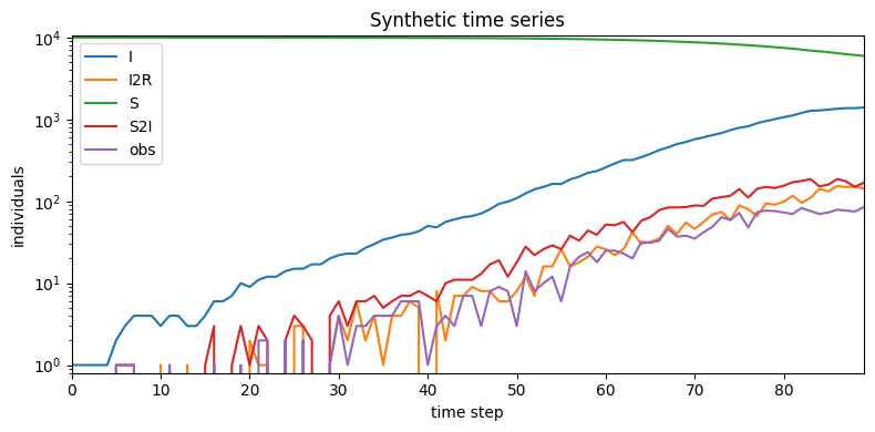
为了检查我们的模型是否生成合理的数据,我们可以创建一个带空数据的模型,并调用模型的 .generate() 方法。该方法首先调用 .global_model(),然后调用 .initialize(),然后根据空数据的长度,为每个时间步调用一次 .transition()。
[3]:
population = 10000
recovery_time = 10.
empty_data = [None] * 90
model = SimpleSIRModel(population, recovery_time, empty_data)

# We'll repeatedly generate data until a desired number of infections is found.
pyro.set_rng_seed(20200709)
for attempt in range(100):
    synth_data = model.generate({"R0": 2.0})
    total_infections = synth_data["S2I"].sum().item()
    if 4000 <= total_infections <= 6000:
        break
print("Simulated {} infections after {} attempts".format(total_infections, 1 + attempt))
Simulated 4055.0 infections after 6 attempts
生成的数据包含全局变量和时间序列,打包成张量。
[4]:
for key, value in sorted(synth_data.items()):
    print("{}.shape = {}".format(key, tuple(value.shape)))
I.shape = (90,)
I2R.shape = (90,)
R0.shape = ()
S.shape = (90,)
S2I.shape = (90,)
obs.shape = (90,)
rho.shape = ()
[5]:
plt.figure(figsize=(8,4))
for name, value in sorted(synth_data.items()):
    if value.dim():
        plt.plot(value, label=name)
plt.xlim(0, len(empty_data) - 1)
plt.ylim(0.8, None)
plt.xlabel("time step")
plt.ylabel("individuals")
plt.yscale("log")
plt.legend(loc="best")
plt.title("Synthetic time series")
plt.tight_layout()
推断
接下来,我们仅根据观测值 obs 来恢复潜变量的估计。为此,我们将从合成观测值创建一个新的模型实例。
[6]:
obs = synth_data["obs"]
model = SimpleSIRModel(population, recovery_time, obs)
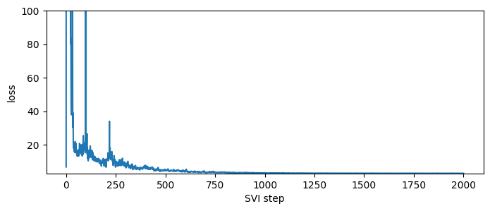
CompartmentalModel 提供了多种推断算法。最便宜且最具可扩展性的算法是 SVI,可通过 .fit_svi() 方法获得。该方法返回一个损失列表,帮助我们诊断收敛性;拟合的参数存储在模型对象中。
[7]:
%%time
losses = model.fit_svi(num_steps=101 if smoke_test else 2001,
                       jit=True)
INFO     Heuristic init: R0=1.83, rho=0.546
INFO     Running inference...
INFO     step 0 loss = 6.808
INFO     step 200 loss = 9.099
INFO     step 400 loss = 7.384
INFO     step 600 loss = 4.401
INFO     step 800 loss = 3.428
INFO     step 1000 loss = 3.242
INFO     step 1200 loss = 3.13
INFO     step 1400 loss = 3.016
INFO     step 1600 loss = 3.029
INFO     step 1800 loss = 3.05
INFO     step 2000 loss = 3.017
INFO     SVI took 12.7 seconds, 157.9 step/sec
CPU times: user 12.8 s, sys: 278 ms, total: 13.1 s
Wall time: 13.2 s
[8]:
plt.figure(figsize=(8, 3))
plt.plot(losses)
plt.xlabel("SVI step")
plt.ylabel("loss")
plt.ylim(min(losses), max(losses[50:]));
推断后,潜变量样本存储在 .samples 属性中。这些主要用于内部使用,不包含全部潜变量。
[9]:
for key, value in sorted(model.samples.items()):
    print("{}.shape = {}".format(key, tuple(value.shape)))
R0.shape = (100, 1)
auxiliary.shape = (100, 1, 2, 90)
rho.shape = (100, 1)
预测
推断后,我们可以使用 .predict() 方法检查潜变量并进行前向预测。首先,我们只预测潜变量。
[10]:
%%time
samples = model.predict()
INFO Predicting latent variables for 90 time steps...
CPU times: user 113 ms, sys: 2.82 ms, total: 116 ms
Wall time: 115 ms
[11]:
for key, value in sorted(samples.items()):
    print("{}.shape = {}".format(key, tuple(value.shape)))
I.shape = (100, 90)
I2R.shape = (100, 90)
R0.shape = (100, 1)
S.shape = (100, 90)
S2I.shape = (100, 90)
auxiliary.shape = (100, 1, 2, 90)
obs.shape = (100, 90)
rho.shape = (100, 1)
[12]:
names = ["R0", "rho"]
fig, axes = plt.subplots(2, 1, figsize=(5, 5))
axes[0].set_title("Posterior estimates of global parameters")
for ax, name in zip(axes, names):
    truth = synth_data[name]
    sns.distplot(samples[name], ax=ax, label="posterior")
    ax.axvline(truth, color="k", label="truth")
    ax.set_xlabel(name)
    ax.set_yticks(())
    ax.legend(loc="best")
plt.tight_layout()
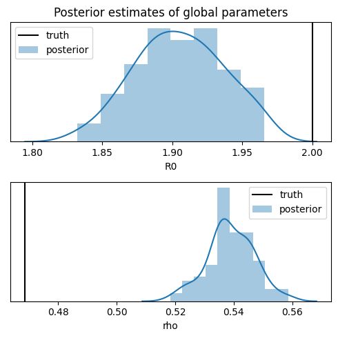
注意,虽然推断恢复了基本再生数 R0,但它对响应率 rho 的估计不佳,并且低估了其不确定性。虽然完美的推断会提供更好的不确定性估计,但众所周知,从数据中恢复响应率是困难的。理想情况下,模型可以引入更窄的先验,这可以通过测试随机人群样本获得,或者通过更准确的观测获得,例如,统计死亡人数而不是确诊感染人数。
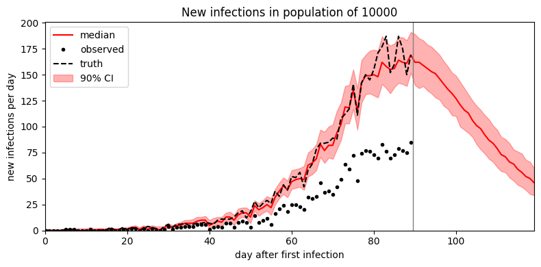
预报
我们可以通过向 .predict() 方法传递一个 forecast 参数来向前预报,指定我们希望预报的时间步数。返回的 sample 将包含第一个观测时间间隔(这里是 90 天)和预报窗口(例如 30 天)期间的时间值。
[13]:
%time
samples = model.predict(forecast=30)
INFO     Predicting latent variables for 90 time steps...
INFO     Forecasting 30 steps ahead...
CPU times: user 2 µs, sys: 1 µs, total: 3 µs
Wall time: 5.96 µs
[14]:
def plot_forecast(samples):
    duration = len(empty_data)
    forecast = samples["S"].size(-1) - duration
    num_samples = len(samples["R0"])

    time = torch.arange(duration + forecast)
    S2I = samples["S2I"]
    median = S2I.median(dim=0).values
    p05 = S2I.kthvalue(int(round(0.5 + 0.05 * num_samples)), dim=0).values
    p95 = S2I.kthvalue(int(round(0.5 + 0.95 * num_samples)), dim=0).values

    plt.figure(figsize=(8, 4))
    plt.fill_between(time, p05, p95, color="red", alpha=0.3, label="90% CI")
    plt.plot(time, median, "r-", label="median")
    plt.plot(time[:duration], obs, "k.", label="observed")
    plt.plot(time[:duration], synth_data["S2I"], "k--", label="truth")
    plt.axvline(duration - 0.5, color="gray", lw=1)
    plt.xlim(0, len(time) - 1)
    plt.ylim(0, None)
    plt.xlabel("day after first infection")
    plt.ylabel("new infections per day")
    plt.title("New infections in population of {}".format(population))
    plt.legend(loc="upper left")
    plt.tight_layout()

plot_forecast(samples)
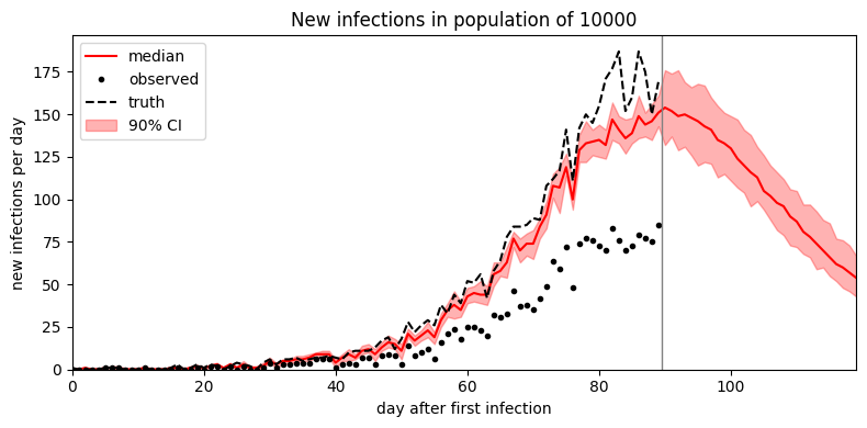
看起来平均场 guide 低估了不确定性。为了改善不确定性估计,我们可以尝试 MCMC 推断。在这个简单模型中,MCMC 只比 SVI 慢一点;在更复杂的模型中,MCMC 可能比 SVI 慢几个数量级。
[15]:
%%time
model = SimpleSIRModel(population, recovery_time, obs)
mcmc = model.fit_mcmc(num_samples=4 if smoke_test else 400,
                      jit_compile=True)
INFO     Running inference...
Warmup:   0%|          | 0/800 [00:00, ?it/s]INFO        Heuristic init: R0=2.05, rho=0.437
Sample: 100%|██████████| 800/800 [01:44,  7.63it/s, step size=1.07e-01, acc. prob=0.890]
CPU times: user 1min 43s, sys: 1.2 s, total: 1min 44s
Wall time: 1min 44s
[16]:
samples = model.predict(forecast=30)
plot_forecast(samples)
INFO     Predicting latent variables for 90 time steps...
INFO     Forecasting 30 steps ahead...
高级建模
到目前为止,我们已经了解了如何创建简单的单变量模型,将模型拟合到数据,以及预测和预报未来数据。接下来我们考虑更高级的建模技术
区域模型
流行病学模型的细节程度各不相同。粗粒度的极端是上面看到的单变量聚合模型。细粒度的极端是网络模型,其中跟踪每个个体的状态,感染发生在稀疏图的边缘(pyro.contrib.epidemiology 不实现网络模型)。我们现在考虑一个中间层模型,其中聚合跟踪许多区域(例如,国家或邮政编码)的每个区域,并且感染发生在区域内以及区域对之间。在 Pyro 中,我们使用 plate 对多个区域进行建模。Pyro 的 CompartmentalModel 类不支持通用的 pyro.plate 语法,但它支持用于区域模型的单个特殊 self.region_plate。当且仅当 CompartmentalModel 使用向量 population 初始化时,此 plate 才可用,并且 region_plate 的大小将是 population 向量的长度。
让我们看看示例 RegionalSIRModel
[17]:
class RegionalSIRModel(CompartmentalModel):
    def __init__(self, population, coupling, recovery_time, data):
        duration = len(data)
        num_regions, = population.shape
        assert coupling.shape == (num_regions, num_regions)
        assert (0 <= coupling).all()
        assert (coupling <= 1).all()
        assert isinstance(recovery_time, float)
        assert recovery_time > 1
        if isinstance(data, torch.Tensor):
            # Data tensors should be oriented as (time, region).
            assert data.shape == (duration, num_regions)
        compartments = ("S", "I")  # R is implicit.

        # We create a regional model by passing a vector of populations.
        super().__init__(compartments, duration, population, approximate=("I",))

        self.coupling = coupling
        self.recovery_time = recovery_time
        self.data = data

    def global_model(self):
        # Assume recovery time is a known constant.
        tau = self.recovery_time

        # Assume reproductive number is unknown but homogeneous.
        R0 = pyro.sample("R0", dist.LogNormal(0., 1.))

        # Assume response rate is heterogeneous and model it with a
        # hierarchical Gamma-Beta prior.
        rho_c1 = pyro.sample("rho_c1", dist.Gamma(10, 1))
        rho_c0 = pyro.sample("rho_c0", dist.Gamma(10, 1))
        with self.region_plate:
            rho = pyro.sample("rho", dist.Beta(rho_c1, rho_c0))

        return R0, tau, rho

    def initialize(self, params):
        # Start with a single infection in region 0.
        I = torch.zeros_like(self.population)
        I[0] += 1
        S = self.population - I
        return {"S": S, "I": I}

    def transition(self, params, state, t):
        R0, tau, rho = params

        # Account for infections from all regions. This uses approximate (point
        # estimate) counts I_approx for infection from other regions, but uses
        # the exact (enumerated) count I for infections from one's own region.
        I_coupled = state["I_approx"] @ self.coupling
        I_coupled = I_coupled + (state["I"] - state["I_approx"]) * self.coupling.diag()
        I_coupled = I_coupled.clamp(min=0)  # In case I_approx is negative.
        pop_coupled = self.population @ self.coupling

        with self.region_plate:
            # Sample flows between compartments.
            S2I = pyro.sample("S2I_{}".format(t),
                              infection_dist(individual_rate=R0 / tau,
                                             num_susceptible=state["S"],
                                             num_infectious=I_coupled,
                                             population=pop_coupled))
            I2R = pyro.sample("I2R_{}".format(t),
                              binomial_dist(state["I"], 1 / tau))

            # Update compartments with flows.
            state["S"] = state["S"] - S2I
            state["I"] = state["I"] + S2I - I2R

            # Condition on observations.
            t_is_observed = isinstance(t, slice) or t < self.duration
            pyro.sample("obs_{}".format(t),
                        binomial_dist(S2I, rho),
                        obs=self.data[t] if t_is_observed else None)
与先前的单变量模型的主要区别在于:我们假设 population 是长度为 num_regions 的向量,我们在 region_plate 内部采样所有隔室变量和一些全局变量,并计算 I_coupled 和 pop_coupled 耦合向量,表示考虑区域内和区域间感染后的有效感染人数和人口。在全局变量中,我们出于演示目的选择将 tau 设置为固定的单个数字,R0 设置为所有区域共享的单个潜变量,并将 rho 设置为每个区域可以取不同值的局部潜变量。请注意,虽然 rho 不在区域之间共享,但我们创建了一个分层模型,其中 rho 的父变量在区域之间共享。虽然我们的一些变量是区域全局的,一些是区域局部的,但只有隔室变量既是区域局部的,又是时间相关的;所有其他参数在所有时间都是固定的。有关时间相关的潜变量,请参阅下面的异质模型部分。
请注意,Pyro 的枚举 MCMC 策略(使用 num_quant_bins > 1 调用 .fit_mcmc())需要额外的逻辑来在隔室之间使用平均场近似:我们将 approximate=("I",) 传递给构造函数,并强制隔室通过 state["I_approx"] 而不是 state["I"] 进行交互。SVI 推断或矩匹配 MCMC 推断(使用默认 num_quant_bins=0 调用 .fit_mcmc())不需要此代码。
有关如何使用区域模型生成数据、训练、预测和预报的演示,请参阅 流行病学:区域模型 示例。
系统发生似然
仅凭聚合观测很难识别流行病学参数。然而,结合聚合计数数据和根据病毒基因测序数据重建的病毒系统发生树,可以更准确地识别某些参数,例如超级传播参数 k (Li et al. 2017)。Pyro 实现了一个 CoalescentRateLikelihood 类,用于根据系统发生树(或一批树样本)的统计数据计算群体似然 p(I|phylogeny)。所需的统计数据恰好是每个采样事件(即病毒基因组测序时间)的时间以及二叉系统发生树中基因合并事件的时间;我们分别将这两个向量称为 leaf_times 和 coal_times,其中对于二叉树,len(leaf_times) == 1 + len(coal_times)。Pyro 提供了一个助手函数 bio_phylo_to_times(),用于从 Bio.Phylo 树对象中提取这些统计数据;反过来,Bio.Phylo 可以解析许多系统发生树的文件格式。
让我们看看包含系统发生似然的示例 SuperspreadingSEIRModel。我们将重点关注模型的系统发生部分
class SuperspreadingSEIRModel(CompartmentalModel):
    def __init__(self, population, incubation_time, recovery_time, data, *,
                 leaf_times=None, coal_times=None):
        compartments = ("S", "E", "I")  # R is implicit.
        duration = len(data)
        super().__init__(compartments, duration, population)
        ...
        self.coal_likelihood = dist.CoalescentRateLikelihood(
            leaf_times, coal_times, duration)
    ...

    def transition(self, params, state, t):
        ...
        # Condition on observations.
        t_is_observed = isinstance(t, slice) or t < self.duration
        R = R0 * state["S"] / self.population
        coal_rate = R * (1. + 1. / k) / (tau_i * state["I"] + 1e-8)
        pyro.factor("coalescent_{}".format(t),
                    self.coal_likelihood(coal_rate, t)
                    if t_is_observed else torch.tensor(0.))
我们首先构建了一个 CoalescentRateLikelihood 对象,用于整个推断和预测过程;这只需进行一次预处理工作,因此评估 self.coal_likelihood(...) 的成本很低。请注意,(leaf_times, coal_times) 应以时间步为单位,与时间索引 t 和 duration 相同。通常 leaf_times 在 [0, duration) 范围内,但 coal_times 在 leaf_times 之前(作为共同祖先点),并且可能为负。似然涉及合并过程中的合并率 coal_rate;我们可以从流行病学模型计算出它。在这个超级传播模型中,coal_rate 取决于再生数 R、超级传播参数 k、潜伏期 tau_i 以及当前的感染人数 state["I"] (Li et al. 2017)。
异质模型
流行病学参数通常随时间变化,这是由于人类干预、天气变化和其他外部因素造成的。我们可以通过将静态潜变量从 .global_model() 移动到 .initialize() 和 .transition() 来在 CompartmentalModel 中建模实值随时间变化的潜变量。例如,我们可以通过在一个随机 R0 初始化并乘以漂移因子来建模对数空间中的布朗漂移下的再生数,就像 HeterogeneousSIRModel 示例中所示
class HeterogeneousSIRModel(CompartmentalModel):
    ...
    def global_model(self):
        tau = self.recovery_time
        R0 = pyro.sample("R0", dist.LogNormal(0., 1.))
        rho = ...
        return R0, tau, rho

    def initialize(self, params):
        # Start with a single infection.
        # We also store the initial beta value in the state dict.
        return {"S": self.population - 1, "I": 1, "beta": torch.tensor(1.)}

    def transition(self, params, state, t):
        R0, tau, rho = params
        # Sample heterogeneous variables.
        # This assumes beta slowly drifts via Brownian motion in log space.
        beta = pyro.sample("beta_{}".format(t),
                           dist.LogNormal(state["beta"].log(), 0.1))
        Rt = pyro.deterministic("Rt_{}".format(t), R0 * beta)

        # Sample flows between compartments.
        S2I = pyro.sample("S2I_{}".format(t),
                          infection_dist(individual_rate=Rt / tau,
                                         num_susceptible=state["S"],
                                         num_infectious=state["I"],
                                         population=self.population))
        ...
        # Update compartments and heterogeneous variables.
        state["S"] = state["S"] - S2I
        state["I"] = state["I"] + S2I - I2R
        state["beta"] = beta  # We store the latest beta value in the state dict.
        ...
这里我们在 .initialize() 中确定性地初始化一个比例因子 beta = 1,然后让它通过对数布朗运动漂移。我们还需要更新 state["beta"],就像我们更新隔室变量一样。现在,当我们调用 .predict() 时,beta 将作为时间序列提供。虽然我们可以写成 Rt = R0 * beta,但我们 instead 将此计算包装在 pyro.deterministic 中,从而将 Rt 作为 .predict() 提供的另一个时间序列暴露出来。请注意,我们可以选择在 .initialize() 中采样 R0 并让 Rt 直接漂移,而不是引入比例因子 beta。然而,将两者分离为非中心化形式可以改善几何结构 (Betancourt and Girolami 2013)。
传入随时间变化的协变量作为张量也很容易,就像我们向所有示例模型的构造函数传递 data 一样。要预测不同因果干预的影响,您可以传入一个比 duration 更长的协变量,运行推断(仅查看前 [0,duration) 条目),然后修改 duration 之后的协变量条目,并生成不同的 .predict() 结果。
复杂隔室流
CompartmentalModel 类默认假定隔室呈线性排列,并在名为“R”的隐式终端隔室中终止,例如 S-I-R、S-E-I-R 或箱式模型,如 S-E1-E2-I1-I2-I3-R。要描述隔室之间更复杂的流动,您可以重写 .compute_flows() 方法。但是,目前不支持带无向循环(例如 S-I-S)的流动。
让我们创建一个可能包含以下流动的分支 SIRD 模型
S → I → R
      ↘
        D
与其他模型一样,我们将保留隐式的“R”状态(尽管我们也可以保留隐式的“D”状态和显式的“R”状态)。在 .compute_flows() 方法中,我们将输入一对状态,并且需要计算三个流动值:S2I、I2R 和 I2D。
class SIRDModel(CompartmentalModel):
    def __init__(self, population, data):
        compartments = ("S", "I", "D")
        duration = len(data)
        super().__init__(compartments, duration, population)
        self.data = data

    def compute_flows(self, prev, curr, t):
        S2I = prev["S"] - curr["S"]  # S can only go in one direction.
        I2D = curr["D"] - prev["D"]  # D can only have come from one direction.
        # Now by conservation at I, change + inflows + outflows = 0,
        # so we can solve for the single unknown I2R.
        I2R = prev["I"] - curr["I"] + S2I - I2D
        return {
            "S2I_{}".format(t): S2I,
            "I2D_{}".format(t): I2D,
            "I2R_{}".format(t): I2R,
        }
    ...
    def transition(self, params, state, t):
        ...
        # Sample flows between compartments.
        S2I = pyro.sample("S2I_{}".format(t), ...)
        I2D = pyro.sample("I2D_{}".format(t), ...)
        I2R = pyro.sample("I2R_{}".format(t), ...)

        # Update compartments with flows.
        state["S"] = state["S"] - S2I
        state["I"] = state["I"] + S2I - I2D - I2R
        state["D"] = state["D"] + I2D
        ...
注意,您可以随意命名字典键,只要它们与 .transition() 中的采样语句匹配,并且您在 .transition() 中正确地反转了流计算。在推断期间,Pyro 将检查 .compute_flows() 和 .transition() 计算是否一致。注意避免就地 PyTorch 操作,因为它们会修改张量而不是字典。
+ state["S"] = state["S"] - S2I  # Correct
- state["S"] -= S2I              # AVOID: may corrupt tensors
对于一个稍微复杂一点的例子,请查看 SimpleSEIRDModel。
参考文献
Lucy M. Li, Nicholas C. Grassly, Christophe Fraser (2017) “结合病原体系统发育和发病率时间序列量化传播异质性” https://academic.oup.com/mbe/article/34/11/2982/3952784
Betancourt, Mark Girolami (2013) “分层模型的哈密顿蒙特卡洛方法” https://arxiv.org/abs/1312.0906
[ ]: