scANVI:使用 Pyro 对单细胞数据进行深度生成建模
在本教程中,我们将展示如何使用 Pyro 构建一个用于转录组数据的半监督深度生成模型,该模型可用于将标签从少量已标记细胞传播到大量未标记细胞。具体来说,我们使用 10x Genomics 的外周血单核细胞 (PBMC) 数据集,并(大致)复现了《使用深度生成模型对单细胞转录组数据进行概率性协调和注释》中图 6 的结果。
(请注意,以下代码也可作为脚本获取。)
[1]:
# setup environment
import os
smoke_test = ('CI' in os.environ)  # for continuous integration tests

if not smoke_test:
    # install scanpy (used for pre-processing and UMAP)
    !pip install -q scanpy==1.8.2
    !pip install -q umap-learn==0.5.1
    # install scvi (used to get data)
    !pip install -q scvi-tools[tutorials]
[2]:
# various import statements
import numpy as np

import torch
import torch.nn as nn
from torch.nn.functional import softplus, softmax
from torch.distributions import constraints
from torch.optim import Adam

import pyro
import pyro.distributions as dist
import pyro.poutine as poutine
from pyro.distributions.util import broadcast_shape
from pyro.optim import MultiStepLR
from pyro.infer import SVI, config_enumerate, TraceEnum_ELBO
from pyro.contrib.examples.scanvi_data import get_data

import matplotlib.pyplot as plt
from matplotlib.patches import Patch
数据预处理
[3]:
%%capture
# Download and pre-process data
batch_size = 100
if not smoke_test:
    dataloader, num_genes, l_mean, l_scale, anndata = get_data(dataset='pbmc', cuda=True, batch_size=batch_size)
else:
    dataloader, num_genes, l_mean, l_scale, anndata = get_data(dataset='mock')
OMP: Info #271: omp_set_nested routine deprecated, please use omp_set_max_active_levels instead.
PBMC 转录组数据被编码为一个 N x G 大小的计数矩阵,其中 N=20,000 个细胞,G=21,932 个基因。

[4]:
print("Count data matrix shape:", dataloader.data_x.shape)
print("Mean counts per cell: {:.1f}".format(dataloader.data_x.sum(-1).mean().item()))
Count data matrix shape: torch.Size([20000, 21932])
Mean counts per cell: 1418.6
此外,这 20,000 个细胞中有 200 个已经使用人工整理的标记基因列表进行了标记,其中包括例如 CD4 和 CD8B。这种注释引入了四种离散的细胞类型: - CD8 初始 T 细胞 - CD4 初始 T 细胞 - CD4 记忆 T 细胞 - CD4 调节性 T 细胞
[5]:
print("Number of labeled cells:", dataloader.num_labeled)
Number of labeled cells: 200
半监督生成建模
我们的高层目标是学习一个参数化模型 p(x),该模型能够很好地拟合观测到的计数数据 {x_i}。为了构建一个足够丰富和灵活的模型,我们引入了几个潜变量,这些变量可以捕获数据中的变异性。特别地,我们引入了以下潜变量: - 两个连续潜变量 z_1 和 z_2,用于编码细胞状态等信息 - 一个标量潜变量 ℓ,编码一个细胞中的总计数数量,从而反映细胞大小、捕获效率等 - 一个离散潜变量 y,编码四种可能的细胞标签
我们的模型结构可以用一个板图表示,其中索引 i 遍历 N 个细胞(换句话说,我们正在逐行建模计数矩阵)。特别是,每个细胞都有这些潜变量的独立副本

请注意,在此图中,y 的部分阴影表示 y 有时是未观测到的,有时不是:这是一个半监督模型。
在我们用 Pyro 编写该模型的完整规范(特别是包括神经网络)之前,让我们先写一些代码来演示模型的高层结构
[6]:
def model_sketch(x, y=None):
    # This gene-level parameter modulates the variance of the
    # observation distribution for our vector of counts x
    theta = pyro.param("inverse_dispersion", 10.0 * torch.ones(num_genes),
                       constraint=constraints.positive)

    # The plate statement encodes that each datapoint (i.e. cell count vector x_i)
    # is conditionally independent given its own latent variables.
    with pyro.plate("batch", len(x)):
        # Define a unit Normal prior distribution for z1
        z1 = pyro.sample("z1", dist.Normal(0, torch.ones(latent_dim)).to_event(1))
        # Define a uniform categorical prior for y.
        # Note that if y is None (i.e. y is unobserved) then y will be sampled;
        # otherwise y will be treated as observed.
        y = pyro.sample("y", dist.OneHotCategorical(logits=torch.zeros(num_labels)),
                        obs=y)

        # Pass z1 and y to the z2 decoder neural network
        z2_loc, z2_scale = z2_decoder(z1, y)
        # Define the prior distribution for z2. The parameters of this distribution
        # depend on both z1 and y.
        z2 = pyro.sample("z2", dist.Normal(z2_loc, z2_scale).to_event(1))

        # Define a LogNormal prior distribution for the log count variable ℓ
        l = pyro.sample("l", dist.LogNormal(l_loc, l_scale).to_event(1))

        # We now construct the observation distribution. To do this we
        # first pass z2 to the x decoder neural network.
        gate_logits, mu = x_decoder(z2)
        # Using the outputs of the neural network we can define the parameters
        # of our ZINB observation distribution.
        # Note that by construction mu is normalized (i.e. mu.sum(-1) == 1) and the
        # total scale of counts for each cell is determined by the latent variable ℓ.
        # That is, `l * mu` is a G-dimensional vector of mean gene counts.
        nb_logits = (l * mu).log() - theta.log()
        x_dist = dist.ZeroInflatedNegativeBinomial(gate_logits=gate_logits,
                                                   total_count=theta,
                                                   logits=nb_logits)
        # Observe the datapoint x using the observation distribution x_dist
        pyro.sample("x", x_dist.to_event(1), obs=x)
变分推断
回想一下,在变分推断中,需要指定一个变分分布。在 Pyro 中,我们称之为 guides。虽然 Pyro 包含一些用于自动构建这些分布的机制,但对于复杂的模型,通常需要手动构建它们以获得最佳性能。让我们描绘一下我们用于该模型的 guide 的高层结构
[7]:
# The guide specifies the variational distribution
def guide_sketch(self, x, y=None):
    # This plate statement matches the plate in the model
    with pyro.plate("batch", len(x)):
        # We pass the observed count vector x to an encoder network
        # that generates the parameters we use to define the variational
        # distributions for the latent variables z2 and ℓ.
        z2_loc, z2_scale, l_loc, l_scale = z2l_encoder(x)
        pyro.sample("l", dist.LogNormal(l_loc, l_scale).to_event(1))
        z2 = pyro.sample("z2", dist.Normal(z2_loc, z2_scale).to_event(1))

        # We only need to specify a variational distribution over y if y is unobserved
        if y is None:
            # We use the `classifier` neural network to turn the latent code
            # z2 into logits that we can use to specify a distribution over y.
            y_logits = classifier(z2)
            y_dist = dist.OneHotCategorical(logits=y_logits)
            y = pyro.sample("y", y_dist)

        # Finally we generate the parameters for the z1 distribution by
        # passing z2 and y through an encoder neural network z1_encoder.
        z1_loc, z1_scale = z1_encoder(z2, y)
        pyro.sample("z1", dist.Normal(z1_loc, z1_scale).to_event(1))
定义用于构建全连接神经网络和重塑张量的一些辅助函数
[8]:
# Helper for making fully-connected neural networks
def make_fc(dims):
    layers = []
    for in_dim, out_dim in zip(dims, dims[1:]):
        layers.append(nn.Linear(in_dim, out_dim))
        layers.append(nn.BatchNorm1d(out_dim))
        layers.append(nn.ReLU())
    return nn.Sequential(*layers[:-1])  # Exclude final ReLU non-linearity

# Splits a tensor in half along the final dimension
def split_in_half(t):
    return t.reshape(t.shape[:-1] + (2, -1)).unbind(-2)

# Helper for broadcasting inputs to neural net
def broadcast_inputs(input_args):
    shape = broadcast_shape(*[s.shape[:-1] for s in input_args]) + (-1,)
    input_args = [s.expand(shape) for s in input_args]
    return input_args
神经网络编码器和解码器
完成模型和 guide 规范的主要工作是定义各种解码器/编码器神经网络。由于这主要只是调用标准 PyTorch API 的问题,我们在此不作详细介绍。我们只快速看一下 XDecoder,这是我们在模型中用于指定观测分布 p(x | z_2) 的解码器神经网络。
[9]:
# Used in parameterizing p(x | z2)
class XDecoder(nn.Module):
    # This __init__ statement is executed once upon construction of the neural network.
    # Here we specify that the neural network has input dimension z2_dim
    # and output dimension 2 * num_genes.
    def __init__(self, num_genes, z2_dim, hidden_dims):
        super().__init__()
        dims = [z2_dim] + hidden_dims + [2 * num_genes]
        self.fc = make_fc(dims)

    # This method defines the actual computation of the neural network. It takes
    # z2 as input and spits out two parameters that are then used in the model
    # to define the ZINB observation distribution. In particular it generates
    # `gate_logits`, which controls zero-inflation, and `mu` which encodes the
    # relative frequencies of different genes.
    def forward(self, z2):
        gate_logits, mu = split_in_half(self.fc(z2))
        # Note that mu is normalized so that total count information is
        # encoded by the latent variable ℓ.
        mu = softmax(mu, dim=-1)
        return gate_logits, mu
现在我们定义其余的编码器和解码器神经网络
[10]:
# Used in parameterizing p(z2 | z1, y)
class Z2Decoder(nn.Module):
    def __init__(self, z1_dim, y_dim, z2_dim, hidden_dims):
        super().__init__()
        dims = [z1_dim + y_dim] + hidden_dims + [2 * z2_dim]
        self.fc = make_fc(dims)

    def forward(self, z1, y):
        z1_y = torch.cat([z1, y], dim=-1)
        # We reshape the input to be two-dimensional so that nn.BatchNorm1d behaves correctly
        _z1_y = z1_y.reshape(-1, z1_y.size(-1))
        hidden = self.fc(_z1_y)
        # If the input was three-dimensional we now restore the original shape
        hidden = hidden.reshape(z1_y.shape[:-1] + hidden.shape[-1:])
        loc, scale = split_in_half(hidden)
        # Here and elsewhere softplus ensures that scale is positive. Note that we generally
        # expect softplus to be more numerically stable than exp.
        scale = softplus(scale)
        return loc, scale

# Used in parameterizing q(z2 | x) and q(l | x)
class Z2LEncoder(nn.Module):
    def __init__(self, num_genes, z2_dim, hidden_dims):
        super().__init__()
        dims = [num_genes] + hidden_dims + [2 * z2_dim + 2]
        self.fc = make_fc(dims)

    def forward(self, x):
        # Transform the counts x to log space for increased numerical stability.
        # Note that we only use this transformation here; in particular the observation
        # distribution in the model is a proper count distribution.
        x = torch.log(1 + x)
        h1, h2 = split_in_half(self.fc(x))
        z2_loc, z2_scale = h1[..., :-1], softplus(h2[..., :-1])
        l_loc, l_scale = h1[..., -1:], softplus(h2[..., -1:])
        return z2_loc, z2_scale, l_loc, l_scale

# Used in parameterizing q(z1 | z2, y)
class Z1Encoder(nn.Module):
    def __init__(self, num_labels, z1_dim, z2_dim, hidden_dims):
        super().__init__()
        dims = [num_labels + z2_dim] + hidden_dims + [2 * z1_dim]
        self.fc = make_fc(dims)

    def forward(self, z2, y):
        # This broadcasting is necessary since Pyro expands y during enumeration (but not z2)
        z2_y = broadcast_inputs([z2, y])
        z2_y = torch.cat(z2_y, dim=-1)
        # We reshape the input to be two-dimensional so that nn.BatchNorm1d behaves correctly
        _z2_y = z2_y.reshape(-1, z2_y.size(-1))
        hidden = self.fc(_z2_y)
        # If the input was three-dimensional we now restore the original shape
        hidden = hidden.reshape(z2_y.shape[:-1] + hidden.shape[-1:])
        loc, scale = split_in_half(hidden)
        scale = softplus(scale)
        return loc, scale

# Used in parameterizing q(y | z2)
class Classifier(nn.Module):
    def __init__(self, z2_dim, hidden_dims, num_labels):
        super().__init__()
        dims = [z2_dim] + hidden_dims + [num_labels]
        self.fc = make_fc(dims)

    def forward(self, x):
        logits = self.fc(x)
        return logits
整合所有部分
此时,我们可以将所有部分整合起来。我们将把 Pyro 模型和 guide 打包成一个 PyTorch nn.Module。我们简要讨论一下在我们上面介绍的高层规范 model_sketch 和 guide_sketch 中被忽略的一些更技术性的问题: - 我们使用 pyro.module 语句将各种神经网络注册到 Pyro(这确保它们的参数得到训练)。 - scANVI 所基于的半监督建模框架在 ELBO 损失函数中包含一个附加项,该附加项确保 classifier 神经网络可以从已标记和未标记数据中学习。这解释了 guide 中出现 pyro.factor 语句的原因,该语句本质上只是添加了一个辅助交叉熵损失项。 - 在下面定义 nb_logits 时,我们使用了一个微调因子 epsilon 以确保数值稳定性。将配备神经网络的灵活模型拟合到高维数据不可避免地需要注意一些数值问题。
[11]:
# Packages the scANVI model and guide as a PyTorch nn.Module
class SCANVI(nn.Module):
    def __init__(self, num_genes, num_labels, l_loc, l_scale,
                 latent_dim=10, alpha=0.01, scale_factor=1.0):
        self.num_genes = num_genes
        self.num_labels = num_labels

        # This is the dimension of both z1 and z2
        self.latent_dim = latent_dim

        # The next two hyperparameters determine the prior over the log_count latent variable `l`
        self.l_loc = l_loc
        self.l_scale = l_scale

        # This hyperparameter controls the strength of the auxiliary classification loss
        self.alpha = alpha
        self.scale_factor = scale_factor

        super().__init__()

        # Setup the various neural networks used in the model and guide
        self.z2_decoder = Z2Decoder(z1_dim=self.latent_dim, y_dim=self.num_labels,
                                    z2_dim=self.latent_dim, hidden_dims=[50])
        self.x_decoder = XDecoder(num_genes=num_genes, hidden_dims=[100], z2_dim=self.latent_dim)
        self.z2l_encoder = Z2LEncoder(num_genes=num_genes, z2_dim=self.latent_dim, hidden_dims=[100])
        self.classifier = Classifier(z2_dim=self.latent_dim, hidden_dims=[50], num_labels=num_labels)
        self.z1_encoder = Z1Encoder(num_labels=num_labels, z1_dim=self.latent_dim,
                                    z2_dim=self.latent_dim, hidden_dims=[50])

        self.epsilon = 0.006

    def model(self, x, y=None):
        # Register various nn.Modules (i.e. the decoder/encoder networks) with Pyro
        pyro.module("scanvi", self)

        # This gene-level parameter modulates the variance of the observation distribution
        theta = pyro.param("inverse_dispersion", 10.0 * x.new_ones(self.num_genes),
                           constraint=constraints.positive)

        # We scale all sample statements by scale_factor so that the ELBO loss function
        # is normalized wrt the number of datapoints and genes.
        # This helps with numerical stability during optimization.
        with pyro.plate("batch", len(x)), poutine.scale(scale=self.scale_factor):
            z1 = pyro.sample("z1", dist.Normal(0, x.new_ones(self.latent_dim)).to_event(1))
            y = pyro.sample("y", dist.OneHotCategorical(logits=x.new_zeros(self.num_labels)),
                            obs=y)

            z2_loc, z2_scale = self.z2_decoder(z1, y)
            z2 = pyro.sample("z2", dist.Normal(z2_loc, z2_scale).to_event(1))

            l_scale = self.l_scale * x.new_ones(1)
            l = pyro.sample("l", dist.LogNormal(self.l_loc, l_scale).to_event(1))

            # Note that by construction mu is normalized (i.e. mu.sum(-1) == 1) and the
            # total scale of counts for each cell is determined by `l`
            gate_logits, mu = self.x_decoder(z2)
            nb_logits = (l * mu + self.epsilon).log() - (theta + self.epsilon).log()
            x_dist = dist.ZeroInflatedNegativeBinomial(gate_logits=gate_logits, total_count=theta,
                                                       logits=nb_logits)
            # Observe the datapoint x using the observation distribution x_dist
            pyro.sample("x", x_dist.to_event(1), obs=x)

    # The guide specifies the variational distribution
    def guide(self, x, y=None):
        pyro.module("scanvi", self)
        with pyro.plate("batch", len(x)), poutine.scale(scale=self.scale_factor):
            z2_loc, z2_scale, l_loc, l_scale = self.z2l_encoder(x)
            pyro.sample("l", dist.LogNormal(l_loc, l_scale).to_event(1))
            z2 = pyro.sample("z2", dist.Normal(z2_loc, z2_scale).to_event(1))

            y_logits = self.classifier(z2)
            y_dist = dist.OneHotCategorical(logits=y_logits)
            if y is None:
                # x is unlabeled so sample y using q(y|z2)
                y = pyro.sample("y", y_dist)
            else:
                # x is labeled so add a classification loss term
                # (this way q(y|z2) learns from both labeled and unlabeled data)
                classification_loss = y_dist.log_prob(y)
                # Note that the negative sign appears because we're adding this term in the guide
                # and the guide log_prob appears in the ELBO as -log q
                pyro.factor("classification_loss", -self.alpha * classification_loss, has_rsample=False)

            z1_loc, z1_scale = self.z1_encoder(z2, y)
            pyro.sample("z1", dist.Normal(z1_loc, z1_scale).to_event(1))
训练
既然我们已经完整地指定了模型和 guide,现在可以通过随机变分推断进行训练了!
[12]:
# Clear Pyro param store so we don't conflict with previous
# training runs in this session
pyro.clear_param_store()
# Fix random number seed
pyro.util.set_rng_seed(0)
# Enable optional validation warnings
pyro.enable_validation(True)

# Instantiate instance of model/guide and various neural networks
scanvi = SCANVI(num_genes=num_genes, num_labels=4,
                l_loc=l_mean, l_scale=l_scale,
                scale_factor=1.0 / (batch_size * num_genes))
if not smoke_test:
    scanvi = scanvi.cuda()

# Setup an optimizer (Adam) and learning rate scheduler.
# We start with a moderately high learning rate (0.006) and
# reduce by a factor of 5 after 20 epochs.
scheduler = MultiStepLR({'optimizer': Adam,
                         'optim_args': {'lr': 0.006},
                         'gamma': 0.2, 'milestones': [20]})

# Tell Pyro to enumerate out y when y is unobserved.
# (By default y would be sampled from the guide)
guide = config_enumerate(scanvi.guide, "parallel", expand=True)

# Setup a variational objective for gradient-based learning.
# Note we use TraceEnum_ELBO in order to leverage Pyro's machinery
# for automatic enumeration of the discrete latent variable y.
elbo = TraceEnum_ELBO(strict_enumeration_warning=False)
svi = SVI(scanvi.model, guide, scheduler, elbo)

# Training loop.
# We train for 80 epochs, although this isn't enough to achieve full convergence.
# For optimal results it is necessary to tweak the optimization parameters.
# For our purposes, however, 80 epochs of training is sufficient.
# Training should take about 8 minutes on a GPU-equipped Colab instance.
num_epochs = 80 if not smoke_test else 1

for epoch in range(num_epochs):
    losses = []

    # Take a gradient step for each mini-batch in the dataset
    for x, y in dataloader:
        if y is not None:
            y = y.type_as(x)
        loss = svi.step(x, y)
        losses.append(loss)

    # Tell the scheduler we've done one epoch.
    scheduler.step()

    print("[Epoch %02d]  Loss: %.5f" % (epoch, np.mean(losses)))

print("Finished training!")
[Epoch 00]  Loss: 0.34436
[Epoch 01]  Loss: 0.21656
[Epoch 02]  Loss: 0.15006
[Epoch 03]  Loss: 0.12347
[Epoch 04]  Loss: 0.10913
[Epoch 05]  Loss: 0.10095
[Epoch 06]  Loss: 0.09812
[Epoch 07]  Loss: 0.09501
[Epoch 08]  Loss: 0.09236
[Epoch 09]  Loss: 0.09102
[Epoch 10]  Loss: 0.08964
[Epoch 11]  Loss: 0.08916
[Epoch 12]  Loss: 0.08763
[Epoch 13]  Loss: 0.08644
[Epoch 14]  Loss: 0.08549
[Epoch 15]  Loss: 0.08450
[Epoch 16]  Loss: 0.08330
[Epoch 17]  Loss: 0.08281
[Epoch 18]  Loss: 0.08258
[Epoch 19]  Loss: 0.08243
[Epoch 20]  Loss: 0.08225
[Epoch 21]  Loss: 0.08222
[Epoch 22]  Loss: 0.08217
[Epoch 23]  Loss: 0.08214
[Epoch 24]  Loss: 0.08211
[Epoch 25]  Loss: 0.08208
[Epoch 26]  Loss: 0.08205
[Epoch 27]  Loss: 0.08201
[Epoch 28]  Loss: 0.08198
[Epoch 29]  Loss: 0.08196
[Epoch 30]  Loss: 0.08193
[Epoch 31]  Loss: 0.08189
[Epoch 32]  Loss: 0.08186
[Epoch 33]  Loss: 0.08183
[Epoch 34]  Loss: 0.08179
[Epoch 35]  Loss: 0.08177
[Epoch 36]  Loss: 0.08174
[Epoch 37]  Loss: 0.08170
[Epoch 38]  Loss: 0.08169
[Epoch 39]  Loss: 0.08166
[Epoch 40]  Loss: 0.08163
[Epoch 41]  Loss: 0.08161
[Epoch 42]  Loss: 0.08160
[Epoch 43]  Loss: 0.08158
[Epoch 44]  Loss: 0.08155
[Epoch 45]  Loss: 0.08153
[Epoch 46]  Loss: 0.08151
[Epoch 47]  Loss: 0.08149
[Epoch 48]  Loss: 0.08149
[Epoch 49]  Loss: 0.08147
[Epoch 50]  Loss: 0.08145
[Epoch 51]  Loss: 0.08143
[Epoch 52]  Loss: 0.08140
[Epoch 53]  Loss: 0.08140
[Epoch 54]  Loss: 0.08138
[Epoch 55]  Loss: 0.08137
[Epoch 56]  Loss: 0.08137
[Epoch 57]  Loss: 0.08134
[Epoch 58]  Loss: 0.08133
[Epoch 59]  Loss: 0.08133
[Epoch 60]  Loss: 0.08130
[Epoch 61]  Loss: 0.08130
[Epoch 62]  Loss: 0.08127
[Epoch 63]  Loss: 0.08127
[Epoch 64]  Loss: 0.08125
[Epoch 65]  Loss: 0.08125
[Epoch 66]  Loss: 0.08124
[Epoch 67]  Loss: 0.08124
[Epoch 68]  Loss: 0.08121
[Epoch 69]  Loss: 0.08120
[Epoch 70]  Loss: 0.08120
[Epoch 71]  Loss: 0.08118
[Epoch 72]  Loss: 0.08119
[Epoch 73]  Loss: 0.08117
[Epoch 74]  Loss: 0.08116
[Epoch 75]  Loss: 0.08114
[Epoch 76]  Loss: 0.08114
[Epoch 77]  Loss: 0.08113
[Epoch 78]  Loss: 0.08111
[Epoch 79]  Loss: 0.08111
Finished training!
绘制结果图
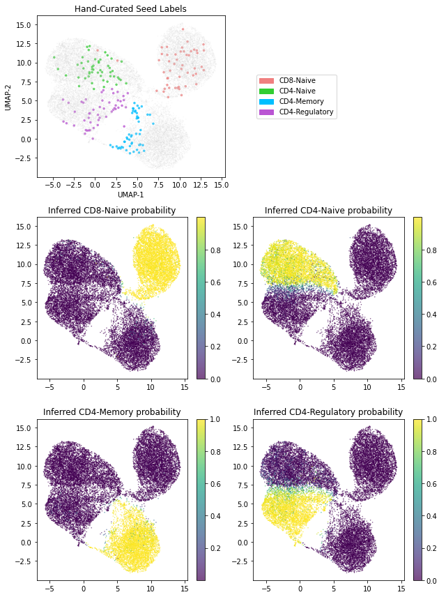
最后,我们生成一个图,展示模型学习到的潜在表示。具体来说,我们将每个细胞与推断出的潜变量 z_2 中编码的 10 维表示相关联。请注意,对于具有计数 x 的给定细胞,可以通过使用我们摊销 guide 中的 z2l_encoder 来计算 z_2 的推断均值。
此外,我们还展示了我们的 classifier 神经网络可以用于标记未标记的细胞。而且,这些标签还带有不确定性估计。
[13]:
if not smoke_test:
    # Now that we're done training we'll inspect the latent representations we've learned
    import scanpy as sc

    # Put the neural networks in evaluation mode (needed because of batch norm)
    scanvi.eval()

    # Compute latent representation (z2_loc) for each cell in the dataset
    latent_rep = scanvi.z2l_encoder(dataloader.data_x)[0]

    # Compute inferred cell type probabilities for each cell
    y_logits = scanvi.classifier(latent_rep)
    # Convert logits to probabilities
    y_probs = softmax(y_logits, dim=-1).data.cpu().numpy()

    # Use scanpy to compute 2-dimensional UMAP coordinates using our
    # learned 10-dimensional latent representation z2
    anndata.obsm["X_scANVI"] = latent_rep.data.cpu().numpy()
    sc.pp.neighbors(anndata, use_rep="X_scANVI")
    sc.tl.umap(anndata)
    umap1, umap2 = anndata.obsm['X_umap'][:, 0], anndata.obsm['X_umap'][:, 1]

    # Construct plots; all plots are scatterplots depicting the two-dimensional UMAP embedding
    # and only differ in how points are colored

    # The topmost plot depicts the 200 hand-curated seed labels in our dataset
    fig, axes = plt.subplots(3, 2, figsize=(9, 12))
    seed_marker_sizes = anndata.obs['seed_marker_sizes']
    axes[0, 0].scatter(umap1, umap2, s=seed_marker_sizes, c=anndata.obs['seed_colors'], marker='.', alpha=0.7)
    axes[0, 0].set_title('Hand-Curated Seed Labels')
    axes[0, 0].set_xlabel('UMAP-1')
    axes[0, 0].set_ylabel('UMAP-2')
    patch1 = Patch(color='lightcoral', label='CD8-Naive')
    patch2 = Patch(color='limegreen', label='CD4-Naive')
    patch3 = Patch(color='deepskyblue', label='CD4-Memory')
    patch4 = Patch(color='mediumorchid', label='CD4-Regulatory')
    axes[0, 1].legend(loc='center left', handles=[patch1, patch2, patch3, patch4])
    axes[0, 1].get_xaxis().set_visible(False)
    axes[0, 1].get_yaxis().set_visible(False)
    axes[0, 1].set_frame_on(False)

    # The remaining plots depict the inferred cell type probability for each of the four cell types
    s10 = axes[1, 0].scatter(umap1, umap2, s=1, c=y_probs[:, 0], marker='.', alpha=0.7)
    axes[1, 0].set_title('Inferred CD8-Naive probability')
    fig.colorbar(s10, ax=axes[1, 0])
    s11 = axes[1, 1].scatter(umap1, umap2, s=1, c=y_probs[:, 1], marker='.', alpha=0.7)
    axes[1, 1].set_title('Inferred CD4-Naive probability')
    fig.colorbar(s11, ax=axes[1, 1])
    s20 = axes[2, 0].scatter(umap1, umap2, s=1, c=y_probs[:, 2], marker='.', alpha=0.7)
    axes[2, 0].set_title('Inferred CD4-Memory probability')
    fig.colorbar(s20, ax=axes[2, 0])
    s21 = axes[2, 1].scatter(umap1, umap2, s=1, c=y_probs[:, 3], marker='.', alpha=0.7)
    axes[2, 1].set_title('Inferred CD4-Regulatory probability')
    fig.colorbar(s21, ax=axes[2, 1])

    fig.tight_layout()