SARS-CoV-2 谱系比例的逻辑增长模型
本 notebook 探讨逻辑增长模型,旨在推断不同 SARS-CoV-2 谱系随时间的差异增长率。在阅读本教程之前,您可能需要熟悉 Pyro 建模基础以及 Pyro 和 PyTorch 中的张量形状。
警告:本教程的目的是演示 Pyro 的建模和推断语法。本教程的**目的不是**对 SARS-CoV-2 进行可靠的推断。
目录
概述
当 SARS-CoV-2 等病毒的不同毒株/谱系/变种在人群中传播时,适应度最高的谱系往往会占据主导地位,而适应度最低的谱系则往往会被适应度最高的谱系淘汰。在本教程中,我们旨在利用 SARS-CoV-2 基因序列的时空数据集来推断不同 SARS-CoV-2 谱系的(差异)增长率。我们将从最简单的模型开始,然后逐步深入到具有层级结构的更复杂模型。
[1]:
import os
import datetime
from functools import partial
import numpy as np
import torch
import pyro
import pyro.distributions as dist
from pyro.infer import SVI, Trace_ELBO
from pyro.infer.autoguide import AutoNormal
from pyro.optim import ClippedAdam
import matplotlib as mpl
import matplotlib.pyplot as plt

if torch.cuda.is_available():
    print("Using GPU")
    torch.set_default_device("cuda")
else:
    print("Using CPU")

smoke_test = ('CI' in os.environ)  # for use in continuous integration testing
Using CPU
加载数据
我们的数据包含数百万条 SARS-CoV-2 病毒基因序列,这些序列被聚类到 PANGO 谱系,并被聚合到全球数百个区域以及 28 天的时间段。预处理由 Nextstrain 的 ncov 工具执行,聚合由 Broad 研究所的 pyro-cov 工具执行。
[2]:
from pyro.contrib.examples.nextstrain import load_nextstrain_counts
dataset = load_nextstrain_counts()

def summarize(x, name=""):
    if isinstance(x, dict):
        for k, v in sorted(x.items()):
            summarize(v, name + "." + k if name else k)
    elif isinstance(x, torch.Tensor):
        print(f"{name}: {type(x).__name__} of shape {tuple(x.shape)} on {x.device}")
    elif isinstance(x, list):
        print(f"{name}: {type(x).__name__} of length {len(x)}")
    else:
        print(f"{name}: {type(x).__name__}")
summarize(dataset)
counts: Tensor of shape (27, 202, 1316) on cpu
features: Tensor of shape (1316, 2634) on cpu
lineages: list of length 1316
locations: list of length 202
mutations: list of length 2634
sparse_counts.index: Tensor of shape (3, 57129) on cpu
sparse_counts.total: Tensor of shape (27, 202) on cpu
sparse_counts.value: Tensor of shape (57129,) on cpu
start_date: datetime
time_step_days: int
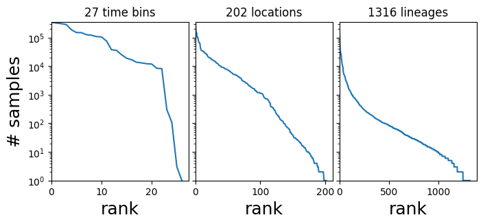
在本教程中,我们关注的是一个三维计数张量 dataset["counts"],其形状为 (T, R, L),其中 T 是时间段的数量,R 是区域的数量,L 是毒株或 PANGO 谱系的数量,dataset["counts"][t,r,l] 是相应时间-区域-位置组合中的样本数量。计数数据严重偏向少数几个大区域和占主导地位的谱系,如 B.1.1.7 和 B.1.617.2。
[3]:
fig, axes = plt.subplots(1, 3, figsize=(8, 3), sharey=True)
for i, name in enumerate(["time bin", "location", "lineage"]):
    counts = dataset["counts"].sum(list({0, 1, 2} - {i}))
    Y = counts.sort(0, True).values
    axes[i].plot(Y)
    axes[i].set_xlim(0, None)
    axes[0].set_ylim(1, None)
    axes[i].set_yscale("log")
    axes[i].set_xlabel(f"rank", fontsize=18)
    axes[i].set_title(f"{len(Y)} {name}s")
axes[0].set_ylabel("# samples", fontsize=18)
plt.subplots_adjust(wspace=0.05);
数据处理辅助函数
[4]:
def get_lineage_id(s):
    """Get lineage id from string name"""
    return np.argmax(np.array([s]) == dataset['lineages'])

def get_location_id(s):
    """Get location id from string name"""
    return np.argmax(np.array([s]) == dataset['locations'])

def get_aggregated_counts_from_locations(locations):
    """Get aggregated counts from a list of locations"""
    return sum([dataset['counts'][:, get_location_id(loc)] for loc in locations])

start = dataset["start_date"]
step = datetime.timedelta(days=dataset["time_step_days"])
date_range = np.array([start + step * t for t in range(len(dataset["counts"]))])
第一个模型
首先,让我们聚焦马萨诸塞州及其周边几个州
[5]:
northeast_states = ['USA / Massachusetts',
                    'USA / New York',
                    'USA / Connecticut',
                    'USA / New Hampshire',
                    'USA / Vermont',
                    'USA / New Jersey',
                    'USA / Maine',
                    'USA / Rhode Island',
                    'USA / Pennsylvania']

northeast_counts = get_aggregated_counts_from_locations(northeast_states)
接下来,让我们提取与世界卫生组织关注的两个变种(WHO variants of concern)对应的子谱系:Alpha 和 Delta
[6]:
# The Alpha and Delta variants include many PANGO lineages, which we need to aggregate.
Q_lineages = [lin for lin in dataset['lineages'] if lin[:2] == 'Q.']
AY_lineages = [lin for lin in dataset['lineages'] if lin[:3] == 'AY.']

alpha_lineages = ['B.1.1.7'] + Q_lineages
delta_lineages = ['B.1.617.2'] + AY_lineages

alpha_ids = [get_lineage_id(lin) for lin in alpha_lineages]
delta_ids = [get_lineage_id(lin) for lin in delta_lineages]

alpha_counts = northeast_counts[:, alpha_ids].sum(-1)
delta_counts = northeast_counts[:, delta_ids].sum(-1)
[7]:
# Let's combine the counts into a single tensor
alpha_delta_counts = torch.stack([alpha_counts, delta_counts]).T
print(alpha_delta_counts.shape)
torch.Size([27, 2])
接下来,让我们绘制计数比例的时间序列(Alpha 对比 Delta)
[8]:
# We skip the first year or so of the pandemic when Alpha and Delta are not present
start_time = 13
total_counts = (alpha_counts + delta_counts)[start_time:]
dates = date_range[start_time:]
plt.figure(figsize=(7, 4))
plt.plot(dates, alpha_counts[start_time:] / total_counts,
         label='Alpha')
plt.plot(dates, delta_counts[start_time:] / total_counts,
         label='Delta')
plt.xlim(min(dates), max(dates))
plt.ylabel("Proportion", fontsize=18)
plt.xticks(rotation=90)
plt.gca().xaxis.set_major_locator(mpl.dates.MonthLocator())
plt.gca().xaxis.set_major_formatter(mpl.dates.DateFormatter("%b %Y"))
plt.legend(fontsize=18)
plt.tight_layout()
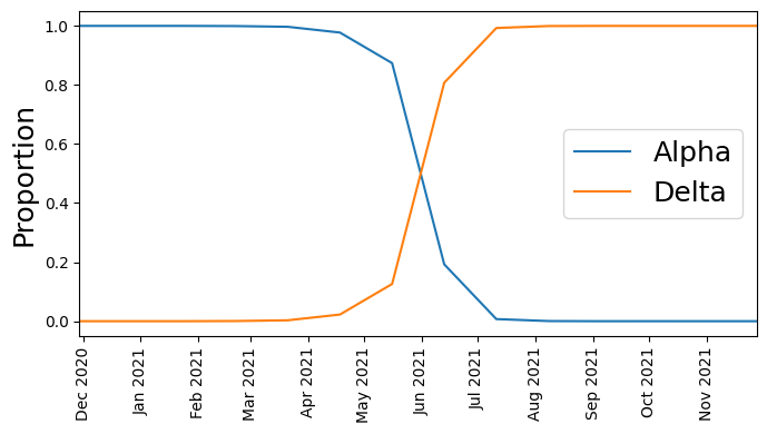
我们看到,起初 Alpha 占主导地位,但随后 Delta 开始超越它,直到 Delta 成为主导。
模型定义
我们不尝试建模观察到的序列总数如何随时间变化(这取决于复杂的人类行为),而是建模每个时间步长中 Alpha 与 Delta 序列的比例。换句话说,如果在给定时间步长我们观察到 8 个 Alpha 谱系和 2 个 Delta 谱系,我们建模的比例是 80% 和 20%,而不是原始计数 8 和 2。为此,我们使用逻辑增长模型,并将多项分布作为似然函数。
[9]:
def basic_model(counts):
    T, L = counts.shape

    # Define plates over lineage and time
    lineage_plate = pyro.plate("lineages", L, dim=-1)
    time_plate = pyro.plate("time", T, dim=-2)

    # Define a growth rate (i.e. slope) and an init (i.e. intercept) for each lineage
    with lineage_plate:
        rate = pyro.sample("rate", dist.Normal(0, 1))
        init = pyro.sample("init", dist.Normal(0, 1))

    # We measure time in units of the SARS-CoV-2 generation time of 5.5 days
    time = torch.arange(float(T)) * dataset["time_step_days"] / 5.5

    # Assume lineages grow linearly in logit space
    logits = init + rate * time[:, None]

    # We use the softmax function (the multivariate generalization of the
    # sigmoid function) to define normalized probabilities from the logits
    probs = torch.softmax(logits, dim=-1)
    assert probs.shape == (T, L)

    # Observe counts via a multinomial likelihood.
    with time_plate:
        pyro.sample(
            "obs",
            dist.Multinomial(probs=probs.unsqueeze(-2), validate_args=False),
            obs=counts.unsqueeze(-2),
        )
让我们看看模型的图形结构
[10]:
pyro.render_model(partial(basic_model, alpha_delta_counts))
[10]:

定义一个用于模型拟合的辅助函数
[11]:
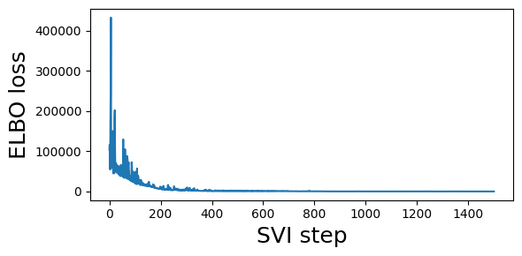
def fit_svi(model, lr=0.1, num_steps=1001, log_every=250):
pyro.clear_param_store() # clear parameters from previous runs
pyro.set_rng_seed(20211214)
if smoke_test:
num_steps = 2
# Define a mean field guide (i.e. variational distribution)
guide = AutoNormal(model, init_scale=0.01)
optim = ClippedAdam({"lr": lr, "lrd": 0.1 ** (1 / num_steps)})
svi = SVI(model, guide, optim, Trace_ELBO())
# Train (i.e. do ELBO optimization) for num_steps iterations
losses = []
for step in range(num_steps):
loss = svi.step()
losses.append(loss)
if step % log_every == 0:
print(f"step {step: >4d} loss = {loss:0.6g}")
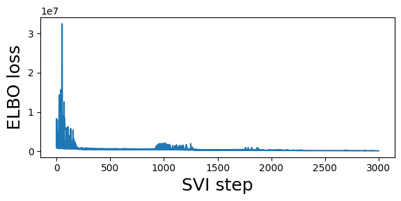
# Plot to assess convergence.
plt.figure(figsize=(6, 3))
plt.plot(losses)
plt.xlabel("SVI step", fontsize=18)
plt.ylabel("ELBO loss", fontsize=18)
plt.tight_layout()
return guide
让我们拟合 basic_model 并检查结果
[12]:
%%time
# We truncate the data to the period with non-zero counts
guide = fit_svi(partial(basic_model, alpha_delta_counts[13:]), num_steps=1501)
step    0 loss = 103782
step  250 loss = 3373.05
step  500 loss = 1299.14
step  750 loss = 524.81
step 1000 loss = 304.319
step 1250 loss = 278.005
step 1500 loss = 261.731
CPU times: user 4.69 s, sys: 29.6 ms, total: 4.72 s
Wall time: 4.73 s
让我们检查隐变量的后验均值:
[13]:
for k, v in guide.median().items():
    print(k, v.data.cpu().numpy())
rate [-0.27021623  0.27021623]
init [ 8.870546 -8.870401]
正如预期的那样,Delta 谱系(对应于索引 1)相对于 Alpha 谱系(对应于索引 0)具有差异增长率优势
[14]:
print("Multiplicative advantage: {:.2f}".format(
      np.exp(guide.median()['rate'][1] - guide.median()['rate'][0])))
Multiplicative advantage: 1.72
这似乎可能是一个高估。我们能否通过分别建模每个空间区域来获得更好的估计?
区域模型
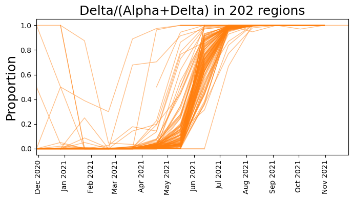
我们不再只关注美国东北部州,而是考虑整个全球数据集,并且不跨区域聚合。
[15]:
# First extract the data we want to use
alpha_counts = dataset['counts'][:, :, alpha_ids].sum(-1)
delta_counts = dataset['counts'][:, :, delta_ids].sum(-1)
counts = torch.stack([alpha_counts, delta_counts], dim=-1)
print("counts.shape: ", counts.shape)
print(f"number of regions: {counts.size(1)}")
counts.shape:  torch.Size([27, 202, 2])
number of regions: 202
[16]:
# We skip the first year or so of the pandemic when Alpha and Delta are not present
start_time = 13
total_counts = (alpha_counts + delta_counts)[start_time:]
dates = date_range[start_time:]
plt.figure(figsize=(7, 4))
plt.plot(dates, delta_counts[start_time:] / total_counts, color="C1", lw=1, alpha=0.5)
plt.xlim(min(dates), max(dates))
plt.ylabel("Proportion", fontsize=18)
plt.xticks(rotation=90)
plt.gca().xaxis.set_major_locator(mpl.dates.MonthLocator())
plt.gca().xaxis.set_major_formatter(mpl.dates.DateFormatter("%b %Y"))
plt.title(f"Delta/(Alpha+Delta) in {counts.size(1)} regions", fontsize=18)
plt.tight_layout()
[17]:
# Model lineage proportions in each region as multivariate logistic growth
def regional_model(counts):
    T, R, L = counts.shape

    # Now we also define a region plate in addition to the time/lineage plates
    lineage_plate = pyro.plate("lineages", L, dim=-1)
    region_plate = pyro.plate("region", R, dim=-2)
    time_plate = pyro.plate("time", T, dim=-3)

    # We use the same growth rate (i.e. slope) for each region
    with lineage_plate:
        rate = pyro.sample("rate", dist.Normal(0, 1))

    # We allow the init to vary from region to region
    init_scale = pyro.sample("init_scale", dist.LogNormal(0, 2))
    with region_plate, lineage_plate:
        init = pyro.sample("init", dist.Normal(0, init_scale))

    # We measure time in units of the SARS-CoV-2 generation time of 5.5 days
    time = torch.arange(float(T)) * dataset["time_step_days"] / 5.5

    # Instead of using the softmax function we directly use the
    # logits parameterization of the Multinomial distribution
    logits = init + rate * time[:, None, None]

    # Observe sequences via a multinomial likelihood.
    with time_plate, region_plate:
        pyro.sample(
            "obs",
            dist.Multinomial(logits=logits.unsqueeze(-2), validate_args=False),
            obs=counts.unsqueeze(-2),
        )
[18]:
pyro.render_model(partial(regional_model, counts))
[18]:

[19]:
%%time
guide = fit_svi(partial(regional_model, counts), num_steps=3001)
step    0 loss = 909278
step  250 loss = 509502
step  500 loss = 630927
step  750 loss = 501493
step 1000 loss = 1.04533e+06
step 1250 loss = 1.98151e+06
step 1500 loss = 328504
step 1750 loss = 279016
step 2000 loss = 310281
step 2250 loss = 217622
step 2500 loss = 204381
step 2750 loss = 176877
step 3000 loss = 152123
CPU times: user 17.3 s, sys: 965 ms, total: 18.3 s
Wall time: 17.3 s
[20]:
print("Multiplicative advantage: {:.2f}".format(
      np.exp(guide.median()['rate'][1] - guide.median()['rate'][0])))
Multiplicative advantage: 1.17
请注意,这比之前的全球估计值要低。
另一种区域模型
我们上面定义的区域模型假定每个谱系的 rate 在区域之间没有变化。在这里,我们添加了额外的层级结构,并允许 rate 在区域之间变化。
[21]:
def regional_model2(counts):
    T, R, L = counts.shape

    lineage_plate = pyro.plate("lineages", L, dim=-1)
    region_plate = pyro.plate("region", R, dim=-2)
    time_plate = pyro.plate("time", T, dim=-3)

    # We assume the init can vary a lot from region to region but
    # that the rate varies considerably less.
    rate_scale = pyro.sample("rate_scale", dist.LogNormal(-4, 2))
    init_scale = pyro.sample("init_scale", dist.LogNormal(0, 2))

    # As before each lineage has a latent growth rate
    with lineage_plate:
        rate_loc = pyro.sample("rate_loc", dist.Normal(0, 1))

    # We allow the rate and init to vary from region to region
    with region_plate, lineage_plate:
        # The per-region per-lineage rate is governed by a hierarchical prior
        rate = pyro.sample("rate",  dist.Normal(rate_loc, rate_scale))
        init = pyro.sample("init", dist.Normal(0, init_scale))

    # We measure time in units of the SARS-CoV-2 generation time of 5.5 days
    time = torch.arange(float(T)) * dataset["time_step_days"] / 5.5
    logits = init + rate * time[:, None, None]

    # Observe sequences via a multinomial likelihood.
    with time_plate, region_plate:
        pyro.sample(
            "obs",
            dist.Multinomial(logits=logits.unsqueeze(-2), validate_args=False),
            obs=counts.unsqueeze(-2),
        )
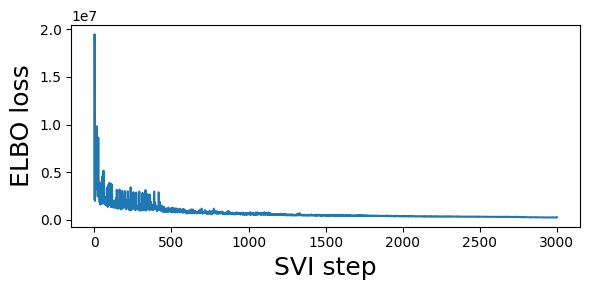
[22]:
pyro.render_model(partial(regional_model2, counts))
[22]:

[23]:
%%time
guide = fit_svi(partial(regional_model2, counts), num_steps=3001)
step    0 loss = 2.14938e+06
step  250 loss = 1.44698e+06
step  500 loss = 1.24936e+06
step  750 loss = 701128
step 1000 loss = 602609
step 1250 loss = 530833
step 1500 loss = 454014
step 1750 loss = 450981
step 2000 loss = 384790
step 2250 loss = 340659
step 2500 loss = 305373
step 2750 loss = 279524
step 3000 loss = 262679
CPU times: user 25 s, sys: 1.05 s, total: 26 s
Wall time: 25.1 s
[24]:
print("Multiplicative advantage: {:.2f}".format(
      (guide.median()['rate_loc'][1] - guide.median()['rate_loc'][0]).exp()))
Multiplicative advantage: 1.14
泛化
到目前为止,我们已经了解了如何一次对两个变种进行全局建模或跨多个区域进行拆分建模,以及如何使用 pyro.plate 对多个变种、区域或时间进行建模。
您还能想到哪些在流行病学上可能合理的模型?这里有一些想法:
您能否建立一个包含两个以上变种的模型,甚至包含所有 PANGO 谱系的模型?
哪些变量应该在谱系之间、区域之间或时间上共享?
您如何处理随时间变化的行为,例如大流行波或疫苗接种?
有关使用此类 SARS-CoV-2 谱系数据构建大型 Pyro 模型的示例,请参阅我们的论文“分析 210 万个 SARS-CoV-2 基因组以识别与传播性相关的突变”(预印本 | 代码),以及使用稍小数据集的贝叶斯工作流教程。
[ ]: