Levy Stable 随机波动率模型¶

本教程通过一个非高斯随机波动率模型的示例，演示了如何使用 Levy Stable 分布进行推理。

Stable 分布的推理非常棘手，因为其密度函数 Stable.log_prob() 计算成本很高。在本教程中，我们将演示三种推理方法：(i) 使用 poutine.reparam 效应将模型转换为可处理的形式，(ii) 在 SVI 中使用无似然损失 EnergyDistance，以及 (iii) 使用包含数值积分对数概率计算的 Stable.log_prob()。

总结¶

Stable.log_prob() 计算成本很高。
Stable 分布的推理需要重参数化或无似然损失。
重参数化
- poutine.reparam() handler 可以使用各种策略转换模型。
- StableReparam 策略可用于 SVI 或 HMC 中的 Stable 分布。
- LatentStableReparam 策略成本稍低，但不能用于似然。
- DiscreteCosineReparam 策略可以改善批量潜在时间序列模型的几何形状。
使用 SVI 的无似然损失
- EnergyDistance 损失允许在 guide 和模型似然中使用 Stable 分布。

目录¶

每日 S&P 数据
使用 EnergyDistance 对对数收益率拟合单个分布
使用以下方法建模随机波动率
- 使用 poutine.reparam 进行重参数化
- 使用 Stable.log_prob() 进行数值积分对数概率

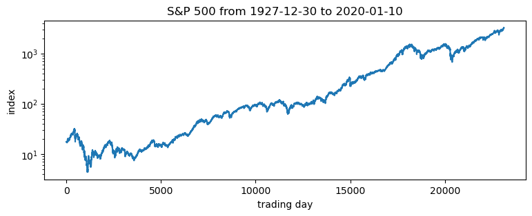
每日 S&P 500 数据¶

以下 S&P 500 每日收盘价从 Yahoo finance 加载。

[1]:

import math
import os
import torch
import pyro
import pyro.distributions as dist
from matplotlib import pyplot
from torch.distributions import constraints

from pyro import poutine
from pyro.contrib.examples.finance import load_snp500
from pyro.infer import EnergyDistance, Predictive, SVI, Trace_ELBO
from pyro.infer.autoguide import AutoDiagonalNormal
from pyro.infer.reparam import DiscreteCosineReparam, StableReparam
from pyro.optim import ClippedAdam
from pyro.ops.tensor_utils import convolve

%matplotlib inline
assert pyro.__version__.startswith('1.9.1')
smoke_test = ('CI' in os.environ)

[2]:

df = load_snp500()
dates = df.Date.to_numpy()
x = torch.tensor(df["Close"]).float()
x.shape

[2]:

torch.Size([23116])

[3]:

pyplot.figure(figsize=(9, 3))
pyplot.plot(x)
pyplot.yscale('log')
pyplot.ylabel("index")
pyplot.xlabel("trading day")
pyplot.title("S&P 500 from {} to {}".format(dates[0], dates[-1]));

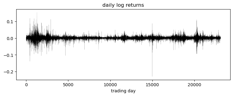
感兴趣的是对数收益率，即连续两天价格对数比率。

[4]:

pyplot.figure(figsize=(9, 3))
r = (x[1:] / x[:-1]).log()
pyplot.plot(r, "k", lw=0.1)
pyplot.title("daily log returns")
pyplot.xlabel("trading day");

[5]:

pyplot.figure(figsize=(9, 3))
pyplot.hist(r.numpy(), bins=200)
pyplot.yscale('log')
pyplot.ylabel("count")
pyplot.xlabel("daily log returns")
pyplot.title("Empirical distribution.  mean={:0.3g}, std={:0.3g}".format(r.mean(), r.std()));

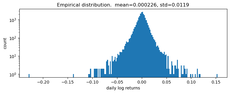
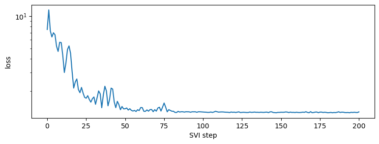
对对数收益率拟合单个分布¶

对数收益率似乎具有重尾。首先，我们尝试对收益率拟合单个分布。为了拟合分布，我们将使用无似然统计推理算法 EnergyDistance，该算法匹配观测数据的分数矩，并且可以处理重尾数据。

[6]:

def model():
    stability = pyro.param("stability", torch.tensor(1.9),
                           constraint=constraints.interval(0, 2))
    skew = 0.
    scale = pyro.param("scale", torch.tensor(0.1), constraint=constraints.positive)
    loc = pyro.param("loc", torch.tensor(0.))
    with pyro.plate("data", len(r)):
        return pyro.sample("r", dist.Stable(stability, skew, scale, loc), obs=r)

[7]:

%%time
pyro.clear_param_store()
pyro.set_rng_seed(1234567890)
num_steps = 1 if smoke_test else 201
optim = ClippedAdam({"lr": 0.1, "lrd": 0.1 ** (1 / num_steps)})
svi = SVI(model, lambda: None, optim, EnergyDistance())
losses = []
for step in range(num_steps):
    loss = svi.step()
    losses.append(loss)
    if step % 20 == 0:
        print("step {} loss = {}".format(step, loss))

print("-" * 20)
pyplot.figure(figsize=(9, 3))
pyplot.plot(losses)
pyplot.yscale("log")
pyplot.ylabel("loss")
pyplot.xlabel("SVI step")
for name, value in sorted(pyro.get_param_store().items()):
    if value.numel() == 1:
        print("{} = {:0.4g}".format(name, value.squeeze().item()))

step 0 loss = 7.497945785522461
step 20 loss = 2.0790653228759766
step 40 loss = 1.6773109436035156
step 60 loss = 1.4146158695220947
step 80 loss = 1.306936502456665
step 100 loss = 1.2835698127746582
step 120 loss = 1.2812254428863525
step 140 loss = 1.2803162336349487
step 160 loss = 1.2787212133407593
step 180 loss = 1.265405535697937
step 200 loss = 1.2878881692886353
--------------------
loc = 0.0002415
scale = 0.008325
stability = 1.982
CPU times: total: 828 ms
Wall time: 2.93 s

[8]:

samples = poutine.uncondition(model)().detach()
pyplot.figure(figsize=(9, 3))
pyplot.hist(samples.numpy(), bins=200)
pyplot.yscale("log")
pyplot.xlabel("daily log returns")
pyplot.ylabel("count")
pyplot.title("Posterior predictive distribution");

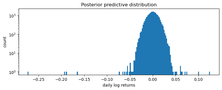
这是一个糟糕的拟合，但这在意料之中，因为我们将所有时间步混合在一起：我们期望这是一个分布（Normal 或 Stable）的尺度混合，但却将其建模为单个分布（在本例中为 Stable）。

建模随机波动率¶

接下来我们将拟合一个随机波动率模型。让我们从一个恒定波动率模型开始，其中对数价格 \(p\) 遵循布朗运动

\[\log p_t = \log p_{t-1} + w_t \sqrt h\]

其中 \(w_t\) 是一系列标准白噪声。我们可以将此模型重写为对数收益率 \(r_t=\log(p_t\,/\,p_{t-1})\) 的形式

\[r_t = w_t \sqrt h\]

现在为了解释波动率聚集，我们可以泛化到随机波动率模型，其中波动率 \(h\) 取决于时间 \(t\)。最简单的此类模型之一是 \(h_t\) 遵循几何布朗运动

\[\log h_t = \log h_{t-1} + \sigma v_t\]

其中 \(v_t\) 再次是一系列标准白噪声。因此，整个模型包含一个几何布朗运动 \(h_t\)，它确定了另一个几何布朗运动 \(p_t\) 的扩散率

\[\begin{split}\log h_t = \log h_{t-1} + \sigma v_t \\ \log p_t = \log p_{t-1} + w_t \sqrt h_t\end{split}\]

通常 \(v_1\) 和 \(w_t\) 都是高斯分布。我们将 \(w_t\) 泛化为 Stable 分布，学习三个参数（稳定性、偏度和位置），但仍然按 \(\sqrt h_t\) 进行缩放。

我们的 Pyro 模型将对增量 \(v_t\) 进行采样，并通过 pyro.deterministic 记录 \(\log h_t\) 的计算。请注意，在 Pyro 中实现此模型有许多方法，并且几何形状可能因实现而异。以下版本与重参数化器结合使用时，似乎具有良好的几何形状。

[9]:

def model(data):
    # Note we avoid plates because we'll later reparameterize along the time axis using
    # DiscreteCosineReparam, breaking independence. This requires .unsqueeze()ing scalars.
    h_0 = pyro.sample("h_0", dist.Normal(0, 1)).unsqueeze(-1)
    sigma = pyro.sample("sigma", dist.LogNormal(0, 1)).unsqueeze(-1)
    v = pyro.sample("v", dist.Normal(0, 1).expand(data.shape).to_event(1))
    log_h = pyro.deterministic("log_h", h_0 + sigma * v.cumsum(dim=-1))
    sqrt_h = log_h.mul(0.5).exp().clamp(min=1e-8, max=1e8)

    # Observed log returns, assumed to be a Stable distribution scaled by sqrt(h).
    r_loc = pyro.sample("r_loc", dist.Normal(0, 1e-2)).unsqueeze(-1)
    r_skew = pyro.sample("r_skew", dist.Uniform(-1, 1)).unsqueeze(-1)
    r_stability = pyro.sample("r_stability", dist.Uniform(0, 2)).unsqueeze(-1)
    pyro.sample("r", dist.Stable(r_stability, r_skew, sqrt_h, r_loc * sqrt_h).to_event(1),
                obs=data)

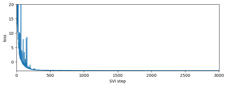
使用重参数化拟合模型¶

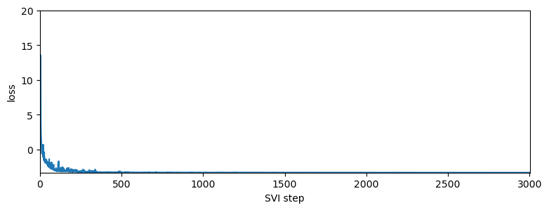
我们使用两个重参数化器：StableReparam 用于处理 Stable 似然（因为 Stable.log_prob() 计算成本很高），以及 DiscreteCosineReparam 用于改善潜在高斯过程 v 的几何形状。然后我们将 reparam_model 用于推理和预测。

[10]:

reparam_model = poutine.reparam(model, {"v": DiscreteCosineReparam(),
                                        "r": StableReparam()})

[11]:

%%time
pyro.clear_param_store()
pyro.set_rng_seed(1234567890)

def fit_model(model):
    num_steps = 1 if smoke_test else 3001
    optim = ClippedAdam({"lr": 0.05, "betas": (0.9, 0.99), "lrd": 0.1 ** (1 / num_steps)})
    guide = AutoDiagonalNormal(model)
    svi = SVI(model, guide, optim, Trace_ELBO())
    losses = []
    stats = []
    for step in range(num_steps):
        loss = svi.step(r) / len(r)
        losses.append(loss)
        stats.append(guide.quantiles([0.325, 0.675]).items())
        if step % 200 == 0:
            median = guide.median()
            print("step {} loss = {:0.6g}".format(step, loss))

    return guide, losses, stats

guide, losses, stats = fit_model(reparam_model)

print("-" * 20)
for name, (lb, ub) in sorted(stats[-1]):
    if lb.numel() == 1:
        lb = lb.squeeze().item()
        ub = ub.squeeze().item()
        print("{} = {:0.4g} ± {:0.4g}".format(name, (lb + ub) / 2, (ub - lb) / 2))

pyplot.figure(figsize=(9, 3))
pyplot.plot(losses)
pyplot.ylabel("loss")
pyplot.xlabel("SVI step")
pyplot.xlim(0, len(losses))
pyplot.ylim(min(losses), 20)

step 0 loss = 2244.54
step 200 loss = -1.16091
step 400 loss = -2.96091
step 600 loss = -3.01823
step 800 loss = -3.03623
step 1000 loss = -3.04261
step 1200 loss = -3.07324
step 1400 loss = -3.06965
step 1600 loss = -3.08399
step 1800 loss = -3.08298
step 2000 loss = -3.08325
step 2200 loss = -3.09142
step 2400 loss = -3.09739
step 2600 loss = -3.10487
step 2800 loss = -3.09952
step 3000 loss = -3.10444
--------------------
h_0 = -0.2587 ± 0.00434
r_loc = 0.04707 ± 0.002965
r_skew = 0.001134 ± 0.0001323
r_stability = 1.946 ± 0.001327
sigma = 0.1359 ± 6.603e-05
CPU times: total: 19.7 s
Wall time: 2min 54s

[11]:

(-3.119090303321589, 20.0)

对数收益率似乎表现出非常小的偏度，但稳定性参数略低于 2，且具有显著差异。这与通常对应于偏度=0 和稳定性=2 的 Normal 模型形成对比。我们现在可以可视化估计的波动率

[12]:

fig, axes = pyplot.subplots(2, figsize=(9, 5), sharex=True)
pyplot.subplots_adjust(hspace=0)
axes[1].plot(r, "k", lw=0.2)
axes[1].set_ylabel("log returns")
axes[1].set_xlim(0, len(r))

# We will pull out median log returns using the autoguide's .median() and poutines.
num_samples = 200
with torch.no_grad():
    pred = Predictive(reparam_model, guide=guide, num_samples=num_samples, parallel=True)(r)
log_h = pred["log_h"]
axes[0].plot(log_h.median(0).values, lw=1)
axes[0].fill_between(torch.arange(len(log_h[0])),
                     log_h.kthvalue(int(num_samples * 0.1), dim=0).values,
                     log_h.kthvalue(int(num_samples * 0.9), dim=0).values,
                     color='red', alpha=0.5)
axes[0].set_ylabel("log volatility")

stability = pred["r_stability"].median(0).values.item()
axes[0].set_title("Estimated index of stability = {:0.4g}".format(stability))
axes[1].set_xlabel("trading day");

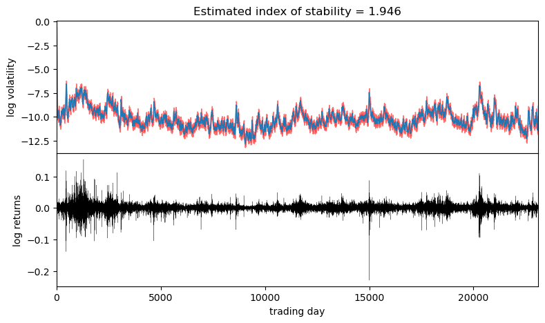
观察到波动率大致遵循对数收益率绝对值较大的区域。请注意，由于我们使用了近似的 AutoDiagonalNormal guide，因此不确定性被低估了。为了获得更精确的不确定性估计，可以使用 HMC 或 NUTS 推理。

使用数值积分对数概率拟合模型¶

我们现在创建一个没有对 Stable 分布进行重参数化的模型。该模型将使用 Stable.log_prob() 方法来计算对数概率密度。

[13]:

from functools import partial
model_with_log_prob = poutine.reparam(model, {"v": DiscreteCosineReparam()})

[14]:

%%time
pyro.clear_param_store()
pyro.set_rng_seed(1234567890)

guide_with_log_prob, losses_with_log_prob, stats_with_log_prob = fit_model(model_with_log_prob)

print("-" * 20)
for name, (lb, ub) in sorted(stats_with_log_prob[-1]):
    if lb.numel() == 1:
        lb = lb.squeeze().item()
        ub = ub.squeeze().item()
        print("{} = {:0.4g} ± {:0.4g}".format(name, (lb + ub) / 2, (ub - lb) / 2))

pyplot.figure(figsize=(9, 3))
pyplot.plot(losses_with_log_prob)
pyplot.ylabel("loss")
pyplot.xlabel("SVI step")
pyplot.xlim(0, len(losses_with_log_prob))
pyplot.ylim(min(losses_with_log_prob), 20)

step 0 loss = 10.872
step 200 loss = -3.21741
step 400 loss = -3.28172
step 600 loss = -3.28264
step 800 loss = -3.28722
step 1000 loss = -3.29258
step 1200 loss = -3.28663
step 1400 loss = -3.30035
step 1600 loss = -3.29928
step 1800 loss = -3.30102
step 2000 loss = -3.30336
step 2200 loss = -3.30392
step 2400 loss = -3.30549
step 2600 loss = -3.30622
step 2800 loss = -3.30624
step 3000 loss = -3.30575
--------------------
h_0 = -0.2038 ± 0.005494
r_loc = 0.04509 ± 0.003355
r_skew = -0.09735 ± 0.02454
r_stability = 1.918 ± 0.002963
sigma = 0.1391 ± 6.794e-05
CPU times: total: 1h 20min 43s
Wall time: 1h 7s

[14]:

(-3.3079991399111877, 20.0)

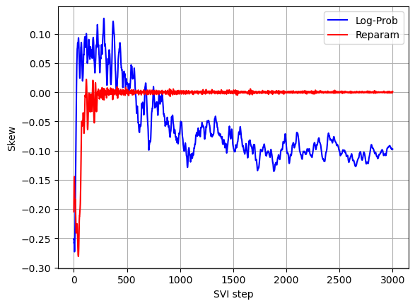
对数收益率表现出负偏度，这在使用 Stable 分布重参数化的模型中没有被捕捉到。负偏度意味着负对数收益率的尾部比正对数收益率的尾部更重。此外，稳定性参数略低于使用 Stable 分布重参数化模型找到的参数（较低的稳定性意味着更重的尾部）。

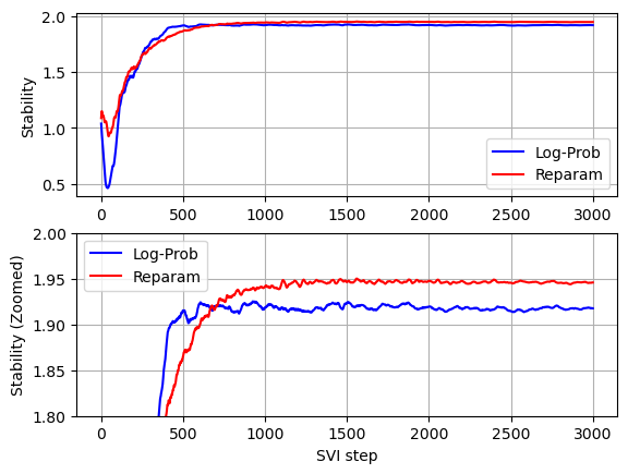
比较两个模型的收敛情况（参见下面的图），我们可以看到，在没有对 Stable 分布进行重参数化的情况下，稳定性参数收敛所需的迭代次数较少，但是由于没有对 Stable 分布进行重参数化时每次迭代的运行时间要高得多，因此总的运行时间显著更高。

[15]:

stability_with_log_prob = []
skew_with_log_prob = []
for stat in stats_with_log_prob:
    stat = dict(stat)
    stability_with_log_prob.append(stat['r_stability'].mean().item())
    skew_with_log_prob.append(stat['r_skew'].mean().item())

stability = []
skew = []
for stat in stats:
    stat = dict(stat)
    stability.append(stat['r_stability'].mean().item())
    skew.append(stat['r_skew'].mean().item())

[16]:

def plot_comparison(log_prob_values, reparam_values, xlabel, ylabel):
    pyplot.plot(log_prob_values, color='b', label='Log-Prob')
    pyplot.plot(reparam_values, color='r', label='Reparam')
    pyplot.xlabel(xlabel)
    pyplot.ylabel(ylabel)
    pyplot.legend(loc='best')
    pyplot.grid()

pyplot.subplot(2,1,1)
plot_comparison(stability_with_log_prob, stability, '', 'Stability')

pyplot.subplot(2,1,2)
plot_comparison(stability_with_log_prob, stability, 'SVI step', 'Stability (Zoomed)')
pyplot.ylim(1.8, 2)

[16]:

(1.8, 2.0)

[17]:

plot_comparison(skew_with_log_prob, skew, 'SVI step', 'Skew')