示例：结合MCMC和SVI使用Predictive和Deterministic¶

在本短教程中，我们将看到如何在模型内部使用deterministic语句，并使用Predictive类检查其样本。此外，还将讨论GammaPoisson分布，因为它将在我们的模型中使用。

查看其他使用Predictive和Deterministic的教程

[1]:

import matplotlib.pyplot as plt
import numpy as np
import pandas as pd
from sklearn.datasets import make_regression
import pyro.distributions as dist
from pyro.infer import MCMC, NUTS, Predictive
from pyro.infer.mcmc.util import summary
from pyro.distributions import constraints
import pyro
import torch

pyro.set_rng_seed(101)

%matplotlib inline
%config InlineBackend.figure_format='retina'

数据生成¶

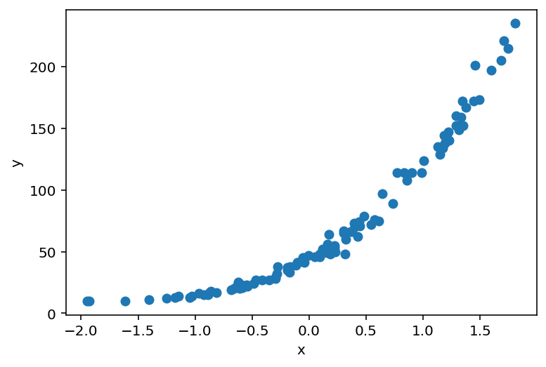
让我们使用sklearn.datasets.make_regression方法生成数据，该方法可以确定特征数量、偏差和噪声功率。我们还将转换目标变量并将其转换为torch张量。

[2]:

X, y = make_regression(n_features=1, bias=150., noise=5., random_state=108)

X_ = torch.tensor(X, dtype=torch.float)
y_ = torch.tensor((y**3)/100000. + 10., dtype=torch.float)
y_.round_().clamp_(min=0);

[3]:

plt.scatter(X_, y_)
plt.ylabel('y')
plt.xlabel('x');

_images/predictive_deterministic_4_0.png

模型定义¶

在我们的模型中，我们首先从零均值和采样标准差的正态分布中采样系数。我们使用to_event(1)将展开维度从batch_shape移动到event_shape，因为我们希望从多元正态分布中采样。deterministic部分用于注册一个name，其value完全由传递给它的参数决定。这里我们使用softplus以确保得到的rate不是负数。然后我们使用plate的向量化版本，将传递的数据集中的counts记录为从GammaPoisson分布中采样得到。

目前这个模型可能有点晦涩，但稍后我们将深入研究采样数据，以更好地理解其内部机制。

[4]:

def model(features, counts):
    N, P = features.shape
    scale = pyro.sample("scale", dist.LogNormal(0, 1))
    coef = pyro.sample("coef", dist.Normal(0, scale).expand([P]).to_event(1))
    rate = pyro.deterministic("rate", torch.nn.functional.softplus(coef @ features.T))
    concentration = pyro.sample("concentration", dist.LogNormal(0, 1))
    with pyro.plate("bins", N):
        return pyro.sample("counts", dist.GammaPoisson(concentration, rate), obs=counts)

推断¶

推断将使用MCMC算法进行。重要提示！请注意，样本字典中只返回scale和coef变量。deterministic部分可以通过Predictive获得，类似于观测到的样本。

[5]:

nuts_kernel = NUTS(model)
mcmc = MCMC(nuts_kernel, num_samples=500)

[6]:

%%time

mcmc.run(X_, y_);

Sample: 100%|██████████| 1000/1000 [00:23, 43.11it/s, step size=6.57e-01, acc. prob=0.922]

CPU times: user 22.8 s, sys: 254 ms, total: 23 s
Wall time: 23.2 s

[7]:

samples = mcmc.get_samples()
for k, v in samples.items():
    print(f"{k}: {tuple(v.shape)}")

coef: (500, 1)
concentration: (500,)
scale: (500,)

[8]:

predictive = Predictive(model, samples)(X_, None)
for k, v in predictive.items():
    print(f"{k}: {tuple(v.shape)}")

counts: (500, 100)
rate: (500, 1, 100)

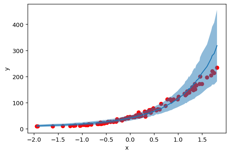
采样后，让我们看看模型与数据的拟合程度。我们计算采样counts的均值和标准差，并将其与原始数据进行绘制。

[9]:

def prepare_counts_df(predictive):
    counts = predictive['counts'].numpy()
    counts_mean = counts.mean(axis=0)
    counts_std = counts.std(axis=0)

    counts_df = pd.DataFrame({
    "feat": X_.squeeze(),
    "mean": counts_mean,
    "high": counts_mean + counts_std,
    "low": counts_mean - counts_std,
    })

    return counts_df.sort_values(by=['feat'])

[10]:

counts_df = prepare_counts_df(predictive)

[11]:

plt.scatter(X_, y_, c='r')
plt.ylabel('y')
plt.xlabel('x')
plt.plot(counts_df['feat'], counts_df['mean'])
plt.fill_between(counts_df['feat'], counts_df['high'], counts_df['low'], alpha=0.5);

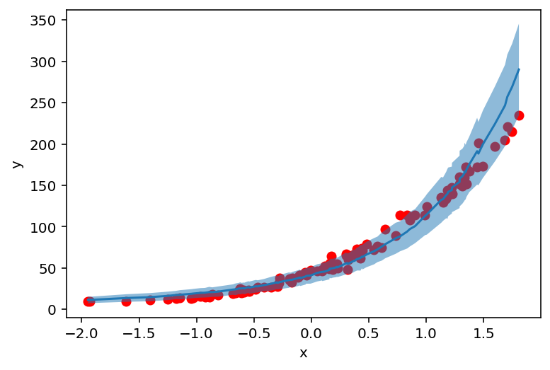
_images/predictive_deterministic_15_0.png

但这些值（和不确定性）从何而来？让我们来找出答案！

检查确定性部分¶

现在让我们来看看本教程的重点。这里使用的GammaPoisson分布，由（concentration, rate）参数化，本质上是NegativeBinomial分布的另一种参数化方式。

NegativeBinomial回答了这个问题：如果在每次试验中获胜的概率是p，那么在看到r次失败（总共）之前，我们将记录多少次成功？

重参数化如下进行

concentration = r
rate = 1 / (p + 1)

首先我们检查concentration和coef变量的采样均值...

[12]:

print('Concentration mean: ', samples['concentration'].mean().item())
print('Concentration std: ', samples['concentration'].std().item())

Concentration mean:  28.77524757385254
Concentration std:  0.7892239689826965

[13]:

print('Coef mean: ', samples['coef'].mean().item())
print('Coef std: ', samples['coef'].std().item())

Coef mean:  -1.2473742961883545
Coef std:  0.036095619201660156

...并进行重参数化（再次请注意我们是从predictive获得的！）。

[14]:

rates = predictive['rate'].squeeze()
rates_reparam = 1. / (rates + 1.) # here's reparametrization

现在我们绘制重参数化的rate

[15]:

fig, (ax1, ax2) = plt.subplots(1, 2)
fig.set_size_inches(13, 4)

ax1.scatter(X_, rates_reparam.mean(axis=0))
ax1.set_ylabel('mean')
ax1.set_xlabel('x')
ax1.set_title('rate means')
ax2.scatter(X_, rates_reparam.std(axis=0))
ax2.set_ylabel('std')
ax2.set_xlabel('x')
ax2.set_title('rate stds');

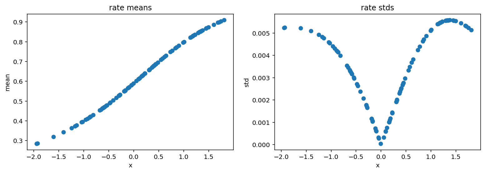
_images/predictive_deterministic_23_0.png

我们看到成功的概率随着x的增加而上升。这意味着在我们观察到由concentration参数决定的28次失败之前，将需要越来越多的试验。

直观上，如果我们想记录28次失败，其中每次失败的概率是0.5，那么也应该需要28次成功。让我们检查一下我们的模型是否遵循这个逻辑

[16]:

fig, (ax1, ax2) = plt.subplots(1, 2)
fig.set_size_inches(13, 4)

ax1.scatter(X_, y_, c='r')
ax1.plot(counts_df['feat'], counts_df['mean'])
ax1.fill_between(counts_df['feat'], counts_df['high'], counts_df['low'], alpha=0.5)
ax1.axhline(samples['concentration'].mean().item(), c='g', linestyle='dashed')
ax1.axvline(-0.46, c='g', linestyle='dashed')
ax1.set_ylabel('y')
ax1.set_xlabel('x')
ax1.set_title('fitted model')
ax2.scatter(X_, rates_reparam.mean(axis=0))
ax2.axhline(0.5, c='g', linestyle='dashed')
ax2.axvline(-0.46, c='g', linestyle='dashed')
ax2.set_ylabel('mean')
ax2.set_xlabel('x')
ax2.set_title('rate means');

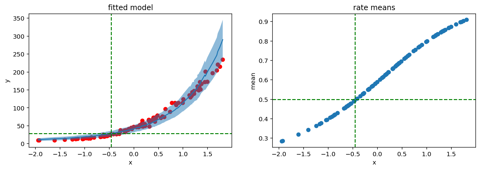
_images/predictive_deterministic_25_0.png

确实如此。红线显示28次成功和率为0.5位于相同的x参数处。

SVI方法¶

Predictive类也可以与SVI方法一起使用。在下一节中，我们将使用AutoGuide的guide以及手动设计的guide。

[17]:

from pyro.infer import SVI, Trace_ELBO
from pyro.optim import Adam
from pyro.infer.autoguide import AutoNormal

手动定义的guide¶

首先我们定义我们的guide，包含模型中所有sample站点，并用可学习参数对其进行参数化。然后我们使用Adam优化器执行梯度下降。

[18]:

def guide(features, counts):
    N, P = features.shape

    scale_param = pyro.param("scale_param", torch.tensor(0.1), constraint=constraints.positive)
    loc_param = pyro.param("loc_param", torch.tensor(0.0))
    scale = pyro.sample("scale", dist.Delta(scale_param))
    coef = pyro.sample("coef", dist.Normal(loc_param, scale).expand([P]).to_event(1))

    concentration_param = pyro.param("concentration_param", torch.tensor(0.1), constraint=constraints.positive)
    concentration = pyro.sample("concentration", dist.Delta(concentration_param))

[19]:

pyro.clear_param_store()

adam_params = {"lr": 0.005, "betas": (0.90, 0.999)}
optimizer = Adam(adam_params)

svi = SVI(model, guide, optimizer, loss=Trace_ELBO())

[20]:

%%time

n_steps = 5001

for step in range(n_steps):
    loss = svi.step(X_, y_)
    if step % 1000 == 0:
        print('Loss: ', loss)

Loss:  4509.724546432495
Loss:  410.72651755809784
Loss:  417.1552972793579
Loss:  395.92131960392
Loss:  447.41201531887054
Loss:  445.11494612693787
CPU times: user 21.2 s, sys: 73.4 ms, total: 21.2 s
Wall time: 21.3 s

Pyro的参数存储包含了将在Predictive阶段使用的学习参数。我们不是提供样本，而是传递guide参数来构建预测分布。

[21]:

list(pyro.get_param_store().items())

[21]:

[('scale_param', tensor(0.1965, grad_fn=<AddBackward0>)),
 ('loc_param', tensor(-1.2427, requires_grad=True)),
 ('concentration_param', tensor(29.1642, grad_fn=<AddBackward0>))]

[22]:

predictive_svi = Predictive(model, guide=guide, num_samples=500)(X_, None)
for k, v in predictive_svi.items():
    print(f"{k}: {tuple(v.shape)}")

scale: (500, 1)
coef: (500, 1, 1)
concentration: (500, 1)
counts: (500, 100)
rate: (500, 1, 100)

[23]:

counts_df = prepare_counts_df(predictive_svi)

[24]:

plt.scatter(X_, y_, c='r')
plt.ylabel('y')
plt.xlabel('x')
plt.plot(counts_df['feat'], counts_df['mean'])
plt.fill_between(counts_df['feat'], counts_df['high'], counts_df['low'], alpha=0.5);

_images/predictive_deterministic_37_0.png

AutoGuide¶

进行SVI的另一种方法是依赖于自动guide生成。这里我们使用AutoNormal，它在底层使用具有对角协方差矩阵的正态分布。

[25]:

pyro.clear_param_store()

adam_params = {"lr": 0.005, "betas": (0.90, 0.999)}
optimizer = Adam(adam_params)

auto_guide = AutoNormal(model)

svi = SVI(model, auto_guide, optimizer, loss=Trace_ELBO())

[26]:

%%time

n_steps = 3001

for step in range(n_steps):
    loss = svi.step(X_, y_)
    if step % 1000 == 0:
        print('Loss: ', loss)

Loss:  3881.8888041973114
Loss:  380.9036132991314
Loss:  375.7684025168419
Loss:  377.94497936964035
CPU times: user 18.8 s, sys: 83.8 ms, total: 18.9 s
Wall time: 19 s

[27]:

auto_guide(X_, y_)

[27]:

{'scale': tensor(1.9367, grad_fn=<ExpandBackward>),
 'coef': tensor([-1.2498], grad_fn=<ExpandBackward>),
 'concentration': tensor(29.5432, grad_fn=<ExpandBackward>)}

当我们检查PARAM_STORE时，我们看到每个sample站点都用正态分布进行近似。

[28]:

list(pyro.get_param_store().items())

[28]:

[('AutoNormal.locs.scale',
  Parameter containing:
  tensor(0.3204, requires_grad=True)),
 ('AutoNormal.scales.scale', tensor(0.5149, grad_fn=<SoftplusBackward>)),
 ('AutoNormal.locs.coef',
  Parameter containing:
  tensor([-1.2510], requires_grad=True)),
 ('AutoNormal.scales.coef', tensor([0.0413], grad_fn=<SoftplusBackward>)),
 ('AutoNormal.locs.concentration',
  Parameter containing:
  tensor(3.3640, requires_grad=True)),
 ('AutoNormal.scales.concentration',
  tensor(0.0299, grad_fn=<SoftplusBackward>))]

最后，我们再次构建预测分布并绘制counts。对于这三种方法，我们都为我们的参数获得了相似的结果。

[29]:

predictive_svi = Predictive(model, guide=auto_guide, num_samples=500)(X_, None)
for k, v in predictive_svi.items():
    print(f"{k}: {tuple(v.shape)}")

scale: (500, 1)
coef: (500, 1, 1)
concentration: (500, 1)
counts: (500, 100)
rate: (500, 1, 100)

[30]:

counts_df = prepare_counts_df(predictive_svi)

[31]:

plt.scatter(X_, y_, c='r')
plt.ylabel('y')
plt.xlabel('x')
plt.plot(counts_df['feat'], counts_df['mean'])
plt.fill_between(counts_df['feat'], counts_df['high'], counts_df['low'], alpha=0.5);

_images/predictive_deterministic_47_0.png