使用动态线性模型 (DLM) 进行预测
在状态空间模型中,动态线性模型 (DLM) 因其可解释性以及能够包含具有动态系数的回归变量而成为最受欢迎的模型之一。Harvey (1989) 和 Durbin and Koopman (2002) 等文献对这些模型进行了完整回顾。本笔记本介绍了通过 Pyro 和 Forecaster 模块构建原生 DLM 的方法。最后,它提供了一个扩展,用于包含灵活的系数先验。
另请参阅:- 预测 II:状态空间模型
工作流程
数据模拟
系数和响应的可视化
标准 DLM 训练和验证
后验比较
留出验证
在不同时间点使用系数先验的 DLM
后验比较
留出验证
[1]:
import matplotlib.pyplot as plt
import pandas as pd
import numpy as np

import torch
import pyro
import pyro.distributions as dist
import pyro.poutine as poutine
from pyro.contrib.forecast import ForecastingModel, Forecaster, eval_crps
from pyro.infer.reparam import LocScaleReparam
from pyro.ops.stats import quantile

%matplotlib inline
assert pyro.__version__.startswith('1.9.1')

pyro.set_rng_seed(20200928)

pd.set_option('display.max_rows', 500)
plt.style.use('fivethirtyeight')
数据模拟
假设我们在时间 \(t\) 有观测值 \(y_t\),满足
其中
\(x_t\) 是时间 \(t\) 的 P x 1 回归变量向量
\(\beta_t\) 是时间 \(t\) 的 P x 1 隐系数向量,服从随机游走分布
\(\epsilon\) 是时间 \(t\) 的噪声
然后我们在以下分布中模拟数据
[2]:
torch.manual_seed(20200101)
# number of predictors, total observations
p = 5
n = 365 * 3

# start, train end, test end
T0 = 0
T1 = n - 28
T2 = n

# initializing coefficients at zeros, simulate all coefficient values
beta0 = torch.empty(n, 1).normal_(0, 0.1).cumsum(0)
betas_p = torch.empty(n, p).normal_(0, 0.02).cumsum(0)
betas = torch.cat([beta0, betas_p], dim=-1)

# simulate regressors
covariates = torch.cat(
    [torch.ones(n, 1), torch.randn(n, p) * 0.1],
    dim=-1
)

# observation with noise
y = ((covariates * betas).sum(-1) + 0.1 * torch.randn(n)).unsqueeze(-1)
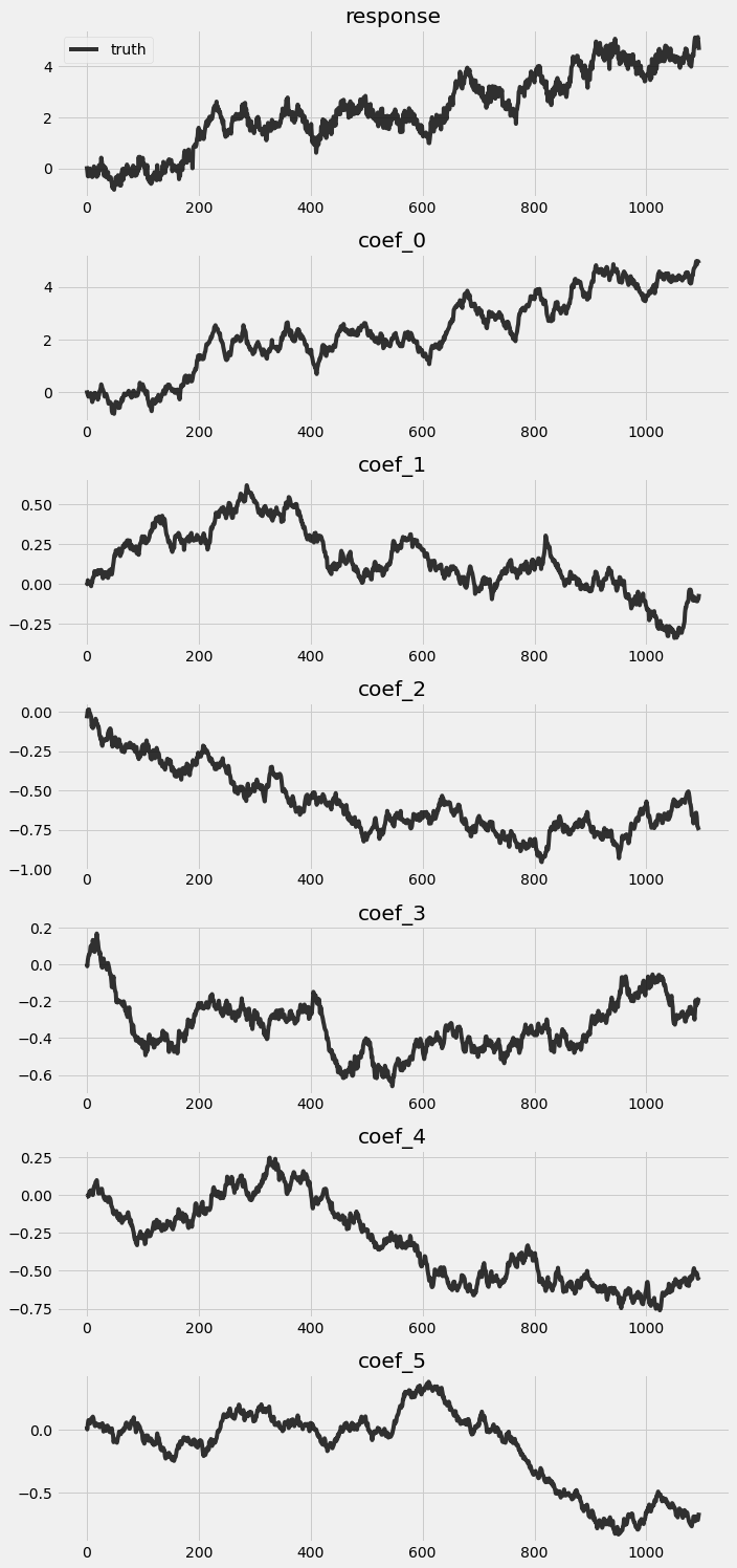
响应和系数的可视化
让我们看一下从前一个块模拟的真实值。
[3]:
fig, axes = plt.subplots(p + 2, 1, figsize=(10, 3 * (p + 2)))
for idx, ax in enumerate(axes):
    if idx == 0:
        axes[0].plot(y, 'k-', label='truth', alpha=.8)
        axes[0].legend()
        axes[0].set_title('response')
    else:
        axes[idx].plot(betas[:, idx -  1], 'k-', label='truth', alpha=.8)
        axes[idx].set_title('coef_{}'.format(idx - 1))
plt.tight_layout()
训练和验证原生 DLM
让我们按照前面讨论的动态构建原生 DLM。
[4]:
class DLM(ForecastingModel):
    def model(self, zero_data, covariates):
        data_dim = zero_data.size(-1)
        feature_dim = covariates.size(-1)

        drift_scale = pyro.sample("drift_scale", dist.LogNormal(-10, 10).expand([feature_dim]).to_event(1))
        with self.time_plate:
            with poutine.reparam(config={"drift": LocScaleReparam()}):
                drift = pyro.sample("drift", dist.Normal(torch.zeros(covariates.size()), drift_scale).to_event(1))

        weight = drift.cumsum(-2)  # A Brownian motion.
        # record in model_trace
        pyro.deterministic("weight", weight)

        prediction = (weight * covariates).sum(-1, keepdim=True)
        assert prediction.shape[-2:] == zero_data.shape
        # record in model_trace
        pyro.deterministic("prediction", prediction)

        scale = pyro.sample("noise_scale", dist.LogNormal(-5, 10).expand([1]).to_event(1))
        noise_dist = dist.Normal(0, scale)

        self.predict(noise_dist, prediction)
[5]:
%%time
pyro.set_rng_seed(1)
pyro.clear_param_store()
model = DLM()
forecaster = Forecaster(
    model,
    y[:T1],
    covariates[:T1],
    learning_rate=0.1,
    learning_rate_decay=0.05,
    num_steps=1000,
)
INFO     step    0 loss = 7.11372e+10
INFO     step  100 loss = 174.352
INFO     step  200 loss = 2.06682
INFO     step  300 loss = 1.27919
INFO     step  400 loss = 1.15015
INFO     step  500 loss = 1.34206
INFO     step  600 loss = 0.928436
INFO     step  700 loss = 1.00953
INFO     step  800 loss = 1.04599
INFO     step  900 loss = 0.870245
CPU times: user 8.16 s, sys: 39.7 ms, total: 8.2 s
Wall time: 8.22 s
后验比较
我们提取样本内期间的后验,并将其与真实值进行比较。
[6]:
pyro.set_rng_seed(1)
# record all latent variables in a trace
with poutine.trace() as tr:
    forecaster(y[:T1], covariates[:T1], num_samples=100)

# extract the values from the recorded trace
posterior_samples = {
    name: site["value"]
    for name, site in tr.trace.nodes.items()
    if site["type"] == "sample"
}
我们也可以可视化样本内后验。
[7]:
# overlay estimations with truth
fig, axes = plt.subplots(p + 2, 1, figsize=(10, 3 * (p + 2)))
# posterior quantiles of latent variables
pred_p10, pred_p50, pred_p90 = quantile(posterior_samples['prediction'], (0.1, 0.5, 0.9)).squeeze(-1)
# posterior quantiles of latent variables
coef_p10, coef_p50, coef_p90 = quantile(posterior_samples['weight'], (0.1, 0.5, 0.9)).squeeze(-1)

for idx, ax in enumerate(axes):
    if idx == 0:
        axes[0].plot(y[:T1], 'k-', label='truth', alpha=.8, lw=1)
        axes[0].plot(pred_p50, 'r-', label='estimate', alpha=.8, lw=1)
        axes[0].fill_between(torch.arange(0, T1), pred_p10, pred_p90, color="red", alpha=.3)
        axes[0].legend()
        axes[0].set_title('response')
    else:
        axes[idx].plot(betas[:T1, idx -  1], 'k-', label='truth', alpha=.8, lw=1)
        axes[idx].plot(coef_p50[:, idx - 1], 'r-', label='estimate', alpha=.8, lw=1)
        axes[idx].fill_between(torch.arange(0, T1), coef_p10[:, idx-1], coef_p90[:, idx-1], color="red", alpha=.3)
        axes[idx].set_title('coef_{}'.format(idx - 1))
plt.tight_layout()
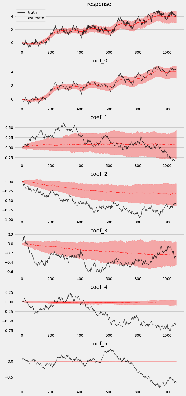
我们可以看到,在原生模型中并非所有系数都能被恢复。
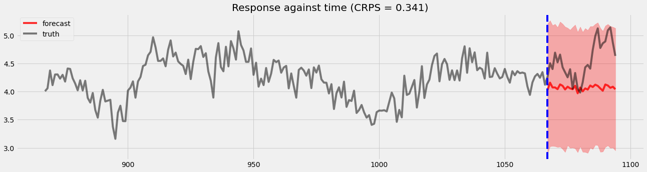
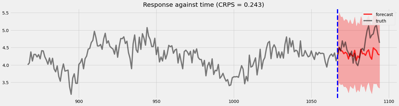
留出验证
在这里,我们将可视化留出验证结果以便后续比较。
[8]:
pyro.set_rng_seed(1)
samples = forecaster(y[:T1], covariates, num_samples=1000)
p10, p50, p90 = quantile(samples, (0.1, 0.5, 0.9)).squeeze(-1)
crps = eval_crps(samples, y[T1:])

plt.figure(figsize=(20, 5))
plt.fill_between(torch.arange(T1, T2), p10, p90, color="red", alpha=.3)
plt.plot(torch.arange(T1, T2), p50, 'r-', label='forecast', alpha=.8)
plt.plot(np.arange(T1 - 200, T2), y[T1 - 200:T2], 'k-', label='truth', alpha=.5)
plt.title("Response against time (CRPS = {:0.3g})".format(crps))
plt.axvline(T1, color='b', linestyle='--')
plt.legend(loc="best");
在不同时间点使用系数先验训练 DLM
有时用户可能对某个时间点的某些系数有先验信念。这在建模者可以为这些系数设置信息性先验的情况下很有用。为了说明,我们创建一些简单的均匀分布的时间点,并使用已知值 \(B_t\) 在这些点上设置先验,如下所示
其中 \(t \in [t_1, t_2, ... t_n]\) 且 \([t_1, t_2, ... t_n]\) 是我们具有经验结果的时间点。
[9]:
# let's provide some priors
time_points = np.concatenate((
    np.arange(300, 320),
    np.arange(600, 620),
    np.arange(900, 920),
))
# broadcast on time-points
priors = betas[time_points, 1:]
[10]:
print(time_points.shape, priors.shape)
(60,) torch.Size([60, 5])
模型训练
现在,让我们构建新的 DLM,它允许用户在某些时间点导入系数先验。
[11]:
class DLM2(ForecastingModel):
    def model(self, zero_data, covariates):
        data_dim = zero_data.size(-1)
        feature_dim = covariates.size(-1)

        drift_scale = pyro.sample("drift_scale", dist.LogNormal(-10, 10).expand([feature_dim]).to_event(1))
        with self.time_plate:
            with poutine.reparam(config={"drift": LocScaleReparam()}):
                drift = pyro.sample("drift", dist.Normal(torch.zeros(covariates.size()), drift_scale).to_event(1))
        weight = drift.cumsum(-2)  # A Brownian motion.
        # record in model_trace
        pyro.deterministic("weight", weight)

        # This is the only change from the simpler DLM model.
        # We inject prior terms as if they were likelihoods using pyro observe statements.
        for tp, prior in zip(time_points, priors):
            pyro.sample("weight_prior_{}".format(tp), dist.Normal(prior, 0.5).to_event(1), obs=weight[..., tp:tp+1, 1:])

        prediction = (weight * covariates).sum(-1, keepdim=True)
        assert prediction.shape[-2:] == zero_data.shape
        # record in model_trace
        pyro.deterministic("prediction", prediction)

        scale = pyro.sample("noise_scale", dist.LogNormal(-5, 10).expand([1]).to_event(1))
        noise_dist = dist.Normal(0, scale)
        self.predict(noise_dist, prediction)
[12]:
%%time
pyro.set_rng_seed(1)
pyro.clear_param_store()
model = DLM2()
forecaster2 = Forecaster(
    model,
    y[:T1],
    covariates[:T1],
    learning_rate=0.1,
    learning_rate_decay=0.05,
    num_steps=1000,
)
INFO     step    0 loss = 7.11372e+10
INFO     step  100 loss = 105.237
INFO     step  200 loss = 2.21884
INFO     step  300 loss = 1.70493
INFO     step  400 loss = 1.64291
INFO     step  500 loss = 1.80583
INFO     step  600 loss = 0.903905
INFO     step  700 loss = 1.25712
INFO     step  800 loss = 1.10254
INFO     step  900 loss = 0.926691
CPU times: user 36.6 s, sys: 316 ms, total: 36.9 s
Wall time: 37.2 s
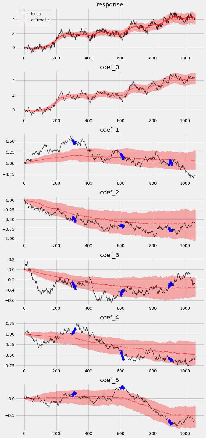
后验比较
最后,让我们重复前一节中的练习,检查样本内后验和留出验证。
[13]:
pyro.set_rng_seed(1)
with poutine.trace() as tr:
    forecaster2(y[:T1], covariates[:T1], num_samples=100)

posterior_samples2 = {
    name: site["value"]
    for name, site in tr.trace.nodes.items()
    if site["type"] == "sample"
}
[14]:
# overlay estimations with truth
fig, axes = plt.subplots(p + 2, 1, figsize=(10, 3 * (p + 2)))
# posterior quantiles of latent variables
pred_p10, pred_p50, pred_p90 = quantile(posterior_samples2['prediction'], (0.1, 0.5, 0.9)).squeeze(-1)
# posterior quantiles of latent variables
coef_p10, coef_p50, coef_p90 = quantile(posterior_samples2['weight'], (0.1, 0.5, 0.9)).squeeze(-1)

for idx, ax in enumerate(axes):
    if idx == 0:
        axes[0].plot(y[:T1], 'k-', label='truth', alpha=.8, lw=1)
        axes[0].plot(pred_p50, 'r-', label='estimate', alpha=.8, lw=1)
        axes[0].fill_between(torch.arange(0, T1), pred_p10, pred_p90, color="red", alpha=.3)
        axes[0].legend()
        axes[0].set_title('response')
    else:
        axes[idx].plot(betas[:T1, idx - 1], 'k-', label='truth', alpha=.8, lw=1)
        axes[idx].plot(coef_p50[:, idx - 1], 'r-', label='estimate', alpha=.8, lw=1)
        if idx >= 2:
            axes[idx].plot(time_points, priors[:, idx-2], 'o', color='blue', alpha=.8, lw=1)
        axes[idx].fill_between(torch.arange(0, T1), coef_p10[:, idx-1], coef_p90[:, idx-1], color="red", alpha=.3)
        axes[idx].set_title('coef_{}'.format(idx - 1))
plt.tight_layout()
留出验证
[15]:
pyro.set_rng_seed(1)
samples2 = forecaster2(y[:T1], covariates, num_samples=1000)
p10, p50, p90 = quantile(samples2, (0.1, 0.5, 0.9)).squeeze(-1)
crps = eval_crps(samples2, y[T1:])
print(samples2.shape, p10.shape)

plt.figure(figsize=(20, 5))
plt.fill_between(torch.arange(T1, T2), p10, p90, color="red", alpha=.3)
plt.plot(torch.arange(T1, T2), p50, 'r-', label='forecast', alpha=.8)
plt.plot(np.arange(T1 - 200, T2), y[T1 - 200:T2], 'k-', label='truth', alpha=.5)
plt.title("Response against time (CRPS = {:0.3g})".format(crps))
plt.axvline(T1, color='b', linestyle='--')
plt.legend(loc="best");
torch.Size([1000, 28, 1]) torch.Size([28])
我们可以看到,在系数运动检测和留出验证方面都有明显的改进。
结论
我们展示了如何使用 Pyro 创建一个经典的 DLM,它提供了不错的预测结果。
通过注入先验,我们在获得更准确的系数和预测方面改进了模型。
参考文献
Harvey, C. A. (1989). Forecasting, Structural Time Series and the Kalman Filter, Cambridge University Press.
Durbin, J., Koopman, S. J.. (2001). Time Series Analysis by State Space Methods, Oxford Statistical Science Series
Scott, S. L., and Varian, H. (2015). “Inferring Causal Impact using Bayesian Structural Time-Series Models” The Annals of Applied Statistics, 9(1), 247–274.
Moore, D., Burnim, J, and the TFP Team (2019). “Structural Time Series modeling in TensorFlow Probability” Available at https://blog.tensorflowcn.cn/2019/03/structural-time-series-modeling-in.html