贝叶斯回归 - 简介(第一部分)
回归是机器学习中最常见和最基本的监督学习任务之一。假设我们有一个数据集 \(\mathcal{D}\),形式如下:
线性回归的目标是将以下形式的函数拟合到数据:
其中 \(w\) 和 \(b\) 是可学习参数,\(\epsilon\) 表示观测噪声。具体来说,\(w\) 是权重矩阵,\(b\) 是偏差向量。
在本教程中,我们将首先在 PyTorch 中实现线性回归,并学习参数 \(w\) 和 \(b\) 的点估计。然后,我们将看到如何通过使用 Pyro 实现贝叶斯回归来将不确定性纳入我们的估计中。此外,我们将学习如何使用 Pyro 的实用函数进行预测以及使用 TorchScript 部署模型。
教程大纲
设置
首先导入所需的模块。
[1]:
%reset -s -f
[2]:
import os
from functools import partial
import torch
import numpy as np
import pandas as pd
import seaborn as sns
import matplotlib.pyplot as plt

import pyro
import pyro.distributions as dist

# for CI testing
smoke_test = ('CI' in os.environ)
assert pyro.__version__.startswith('1.9.1')
pyro.set_rng_seed(1)


# Set matplotlib settings
%matplotlib inline
plt.style.use('default')
数据集
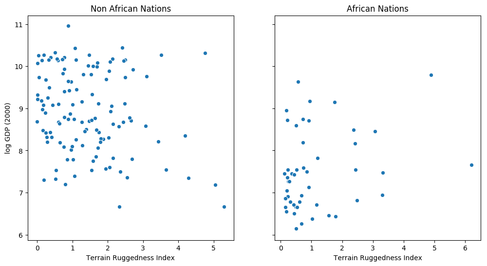
以下示例改编自 [1]。我们希望探索一个国家地形异质性(数据集中变量 rugged 衡量)与其人均 GDP 之间的关系。特别是在 [2] 中,作者注意到地形崎岖或恶劣的地理条件与非洲以外地区较差的经济表现有关,但崎岖地形对非洲国家收入的影响则相反。让我们来看看数据并研究这种关系。我们将重点关注数据集中的三个特征:
rugged:量化地形崎岖度指数cont_africa:给定国家是否位于非洲rgdppc_2000:2000 年实际人均 GDP
响应变量 GDP 是高度偏态的,因此我们将对其进行对数转换。
[3]:
DATA_URL = "https://d2hg8soec8ck9v.cloudfront.net/datasets/rugged_data.csv"
data = pd.read_csv(DATA_URL, encoding="ISO-8859-1")
df = data[["cont_africa", "rugged", "rgdppc_2000"]]
df = df[np.isfinite(df.rgdppc_2000)]
df["rgdppc_2000"] = np.log(df["rgdppc_2000"])
[4]:
fig, ax = plt.subplots(nrows=1, ncols=2, figsize=(12, 6), sharey=True)
african_nations = df[df["cont_africa"] == 1]
non_african_nations = df[df["cont_africa"] == 0]
sns.scatterplot(x=non_african_nations["rugged"],
                y=non_african_nations["rgdppc_2000"],
                ax=ax[0])
ax[0].set(xlabel="Terrain Ruggedness Index",
          ylabel="log GDP (2000)",
          title="Non African Nations")
sns.scatterplot(x=african_nations["rugged"],
                y=african_nations["rgdppc_2000"],
                ax=ax[1])
ax[1].set(xlabel="Terrain Ruggedness Index",
          ylabel="log GDP (2000)",
          title="African Nations");
线性回归
我们希望根据数据集中的两个特征——国家是否位于非洲以及其地形崎岖度指数——来预测一个国家的人均对数 GDP。我们将创建一个简单的类 PyroModule[nn.Linear],它继承自 PyroModule 和 torch.nn.Linear。PyroModule 与 PyTorch 的 nn.Module 非常相似,但它额外支持将 Pyro 基元 作为属性,这些属性可以被 Pyro 的 效果处理程序 (effect handlers) 修改(请参阅下一节,了解如何使模块属性成为 pyro.sample 基元)。一些通用说明如下:
PyTorch 模块中的可学习参数是
nn.Parameter的实例,在本例中是nn.Linear类的weight和bias参数。当在PyroModule中声明为属性时,它们会自动注册到 Pyro 的参数存储中。虽然该模型不需要我们在优化期间约束这些参数的值,但这也可以在PyroModule中使用 PyroParam 语句轻松实现。请注意,虽然
PyroModule[nn.Linear]的forward方法继承自nn.Linear,但它也可以很容易地被覆盖。例如,在逻辑回归的情况下,我们对线性预测值应用 sigmoid 变换。
[5]:
from torch import nn
from pyro.nn import PyroModule

assert issubclass(PyroModule[nn.Linear], nn.Linear)
assert issubclass(PyroModule[nn.Linear], PyroModule)
使用 PyTorch 优化器进行训练
注意,除了两个特征 rugged 和 cont_africa 外,我们的模型中还包含一个交互项,这使得我们可以分别建模崎岖度对非洲内部和外部国家 GDP 的影响。
我们使用均方误差 (MSE) 作为损失函数,并使用 torch.optim 模块中的 Adam 作为优化器。我们希望优化模型的参数,即网络的 weight 和 bias 参数,它们对应于我们的回归系数和截距。
[6]:
# Dataset: Add a feature to capture the interaction between "cont_africa" and "rugged"
df["cont_africa_x_rugged"] = df["cont_africa"] * df["rugged"]
data = torch.tensor(df[["cont_africa", "rugged", "cont_africa_x_rugged", "rgdppc_2000"]].values,
                        dtype=torch.float)
x_data, y_data = data[:, :-1], data[:, -1]

# Regression model
linear_reg_model = PyroModule[nn.Linear](3, 1)

# Define loss and optimize
loss_fn = torch.nn.MSELoss(reduction='sum')
optim = torch.optim.Adam(linear_reg_model.parameters(), lr=0.05)
num_iterations = 1500 if not smoke_test else 2

def train():
    # run the model forward on the data
    y_pred = linear_reg_model(x_data).squeeze(-1)
    # calculate the mse loss
    loss = loss_fn(y_pred, y_data)
    # initialize gradients to zero
    optim.zero_grad()
    # backpropagate
    loss.backward()
    # take a gradient step
    optim.step()
    return loss

for j in range(num_iterations):
    loss = train()
    if (j + 1) % 50 == 0:
        print("[iteration %04d] loss: %.4f" % (j + 1, loss.item()))


# Inspect learned parameters
print("Learned parameters:")
for name, param in linear_reg_model.named_parameters():
    print(name, param.data.numpy())
[iteration 0050] loss: 3179.7852
[iteration 0100] loss: 1616.1371
[iteration 0150] loss: 1109.4117
[iteration 0200] loss: 833.7545
[iteration 0250] loss: 637.5822
[iteration 0300] loss: 488.2652
[iteration 0350] loss: 376.4650
[iteration 0400] loss: 296.0483
[iteration 0450] loss: 240.6140
[iteration 0500] loss: 203.9386
[iteration 0550] loss: 180.6171
[iteration 0600] loss: 166.3493
[iteration 0650] loss: 157.9457
[iteration 0700] loss: 153.1786
[iteration 0750] loss: 150.5735
[iteration 0800] loss: 149.2020
[iteration 0850] loss: 148.5065
[iteration 0900] loss: 148.1668
[iteration 0950] loss: 148.0070
[iteration 1000] loss: 147.9347
[iteration 1050] loss: 147.9032
[iteration 1100] loss: 147.8900
[iteration 1150] loss: 147.8847
[iteration 1200] loss: 147.8827
[iteration 1250] loss: 147.8819
[iteration 1300] loss: 147.8817
[iteration 1350] loss: 147.8816
[iteration 1400] loss: 147.8815
[iteration 1450] loss: 147.8815
[iteration 1500] loss: 147.8815
Learned parameters:
weight [[-1.9478593  -0.20278624  0.39330274]]
bias [9.22308]
绘制回归拟合
让我们分别绘制非洲以外和非洲以内国家的模型回归拟合。
[7]:
fit = df.copy()
fit["mean"] = linear_reg_model(x_data).detach().cpu().numpy()

fig, ax = plt.subplots(nrows=1, ncols=2, figsize=(12, 6), sharey=True)
african_nations = fit[fit["cont_africa"] == 1]
non_african_nations = fit[fit["cont_africa"] == 0]
fig.suptitle("Regression Fit", fontsize=16)
ax[0].plot(non_african_nations["rugged"], non_african_nations["rgdppc_2000"], "o")
ax[0].plot(non_african_nations["rugged"], non_african_nations["mean"], linewidth=2)
ax[0].set(xlabel="Terrain Ruggedness Index",
          ylabel="log GDP (2000)",
          title="Non African Nations")
ax[1].plot(african_nations["rugged"], african_nations["rgdppc_2000"], "o")
ax[1].plot(african_nations["rugged"], african_nations["mean"], linewidth=2)
ax[1].set(xlabel="Terrain Ruggedness Index",
          ylabel="log GDP (2000)",
          title="African Nations");
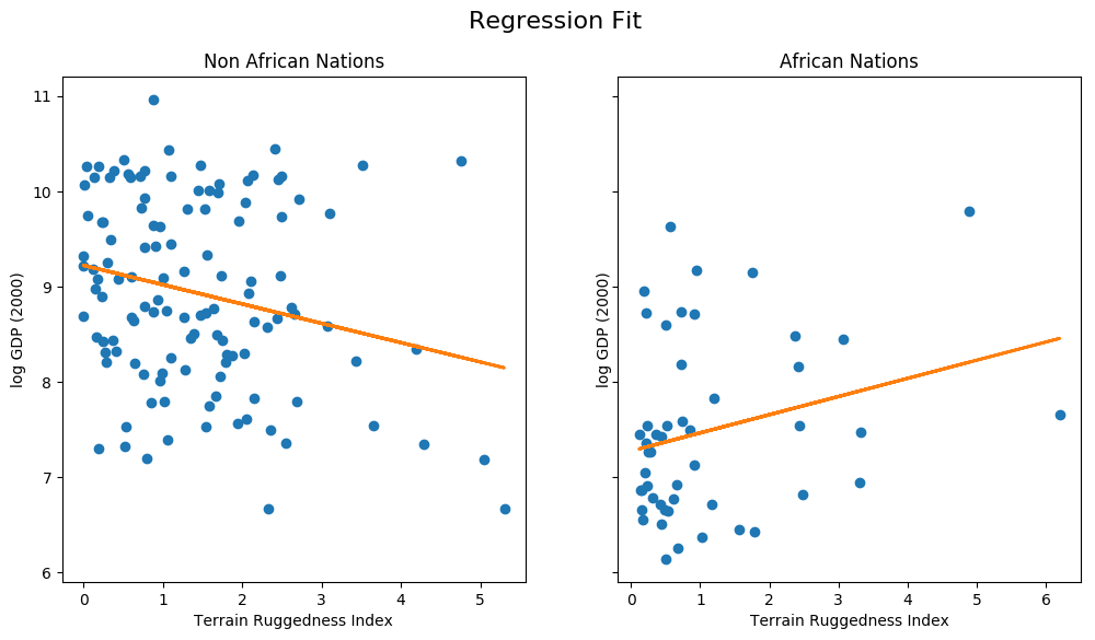
我们注意到地形崎岖度与非非洲国家的 GDP 呈负相关关系,但对非洲国家的 GDP 却有积极影响。然而,这种趋势的稳健性尚不清楚。特别是,我们希望了解由于参数不确定性导致的回归拟合会如何变化。为了解决这个问题,我们将构建一个简单的贝叶斯线性回归模型。贝叶斯建模 提供了一个系统框架,用于推理模型的不确定性。我们不再仅仅学习点估计,而是学习一个与观测数据一致的参数分布。
使用 Pyro 的随机变分推断 (SVI)
模型
为了使我们的线性回归模型成为贝叶斯模型,我们需要为参数 \(w\) 和 \(b\) 设置先验。这些是表示我们关于 \(w\) 和 \(b\) 合理值(在观测任何数据之前)的先验信念的分布。
使用 PyroModule 构建贝叶斯线性回归模型非常直观,如前所述。请注意以下几点:
BayesianRegression模块内部使用相同的PyroModule[nn.Linear]模块。但是,请注意,我们用PyroSample语句替换了该模块的weight和bias参数。这些语句允许我们为weight和bias参数设置先验,而不是将它们视为固定的可学习参数。对于偏置项,我们设置了一个相当宽泛的先验,因为它很可能远高于 0。BayesianRegression.forward方法指定了生成过程。我们通过调用linear模块(正如您所见,它从先验中采样weight和bias参数并返回平均响应值)来生成响应的平均值。最后,我们使用pyro.sample语句的obs参数来条件化观测数据y_data,并学习一个观测噪声sigma。该模型返回由变量mean给出的回归线。
[8]:
from pyro.nn import PyroSample


class BayesianRegression(PyroModule):
    def __init__(self, in_features, out_features):
        super().__init__()
        self.linear = PyroModule[nn.Linear](in_features, out_features)
        self.linear.weight = PyroSample(dist.Normal(0., 1.).expand([out_features, in_features]).to_event(2))
        self.linear.bias = PyroSample(dist.Normal(0., 10.).expand([out_features]).to_event(1))

    def forward(self, x, y=None):
        sigma = pyro.sample("sigma", dist.Uniform(0., 10.))
        mean = self.linear(x).squeeze(-1)
        with pyro.plate("data", x.shape[0]):
            obs = pyro.sample("obs", dist.Normal(mean, sigma), obs=y)
        return mean
使用 AutoGuide
为了进行推断,即学习我们未观测参数的后验分布,我们将使用随机变分推断 (SVI)。Guide 确定了一个分布族,SVI 旨在从这个分布族中找到一个与真实后验的 KL 散度最低的近似后验分布。
用户可以在 Pyro 中编写任意灵活的自定义 guide,但在此教程中,我们将仅限于使用 Pyro 的 autoguide 库。在下一篇教程中,我们将探讨如何手动编写 guide。
首先,我们将使用 AutoDiagonalNormal guide,它将模型中未观测参数的分布建模为具有对角协方差的高斯分布,即它假设潜变量之间没有相关性(正如我们在第二部分中将看到的,这是一个相当强的建模假设)。在底层,这定义了一个 guide,它使用具有可学习参数的 Normal 分布,这些参数对应于模型中的每个 sample 语句。例如,在我们的例子中,这个分布的大小应该是 (5,),对应于每个项的 3 个回归系数,以及截距项和模型中的 sigma 各贡献的 1 个分量。
Autoguide 还支持使用 AutoDelta 学习 MAP 估计,或使用 AutoGuideList 组合 guide(更多信息请参阅文档)。
[9]:
from pyro.infer.autoguide import AutoDiagonalNormal

model = BayesianRegression(3, 1)
guide = AutoDiagonalNormal(model)
优化证据下界
我们将使用随机变分推断 (SVI)(SVI 简介请参阅SVI 第一部分)进行推断。就像在非贝叶斯线性回归模型中一样,我们的训练循环的每次迭代都会进行梯度步进,不同之处在于,在这种情况下,我们将通过构建一个 Trace_ELBO 对象并将其传递给 SVI,来使用证据下界 (ELBO) 目标而不是 MSE 损失。
[10]:
from pyro.infer import SVI, Trace_ELBO


adam = pyro.optim.Adam({"lr": 0.03})
svi = SVI(model, guide, adam, loss=Trace_ELBO())
注意,我们使用 Pyro 的 optim 模块中的 Adam 优化器,而不是像之前那样使用 torch.optim 模块。这里的 Adam 是 torch.optim.Adam 的一个薄包装(讨论请参阅此处)。pyro.optim 中的优化器用于优化和更新 Pyro 参数存储中的参数值。特别是,您会注意到我们无需将可学习参数传递给优化器,因为这由 guide 代码决定并在 SVI 类内部自动发生。要进行 ELBO 梯度步进,我们只需调用 SVI 的 step 方法。我们传递给 SVI.step 的数据参数将同时传递给 model() 和 guide()。完整的训练循环如下所示:
[11]:
pyro.clear_param_store()
for j in range(num_iterations):
    # calculate the loss and take a gradient step
    loss = svi.step(x_data, y_data)
    if j % 100 == 0:
        print("[iteration %04d] loss: %.4f" % (j + 1, loss / len(data)))
[iteration 0001] loss: 6.2310
[iteration 0101] loss: 3.5253
[iteration 0201] loss: 3.2347
[iteration 0301] loss: 3.0890
[iteration 0401] loss: 2.6377
[iteration 0501] loss: 2.0626
[iteration 0601] loss: 1.4852
[iteration 0701] loss: 1.4631
[iteration 0801] loss: 1.4632
[iteration 0901] loss: 1.4592
[iteration 1001] loss: 1.4940
[iteration 1101] loss: 1.4988
[iteration 1201] loss: 1.4938
[iteration 1301] loss: 1.4679
[iteration 1401] loss: 1.4581
我们可以通过从 Pyro 参数存储中获取来检查优化后的参数值。
[12]:
guide.requires_grad_(False)

for name, value in pyro.get_param_store().items():
    print(name, pyro.param(name))
AutoDiagonalNormal.loc Parameter containing:
tensor([-2.2371, -1.8097, -0.1691,  0.3791,  9.1823])
AutoDiagonalNormal.scale tensor([0.0551, 0.1142, 0.0387, 0.0769, 0.0702])
正如您所见,我们现在不仅有学习参数的点估计,还有不确定性估计(AutoDiagonalNormal.scale)。请注意,Autoguide 将潜变量打包到一个张量中,在本例中,模型的每个采样变量对应一个条目。正如我们之前指出的,loc 和 scale 参数的大小都是 (5,),对应于模型中的每个潜变量。
为了更清晰地查看潜参数的分布,我们可以使用 AutoDiagonalNormal.quantiles 方法,该方法将从 autoguide 中解包潜样本,并自动将其约束到 site 的支持域(例如,变量 sigma 必须在 (0, 10) 范围内)。我们看到参数的中位数非常接近我们从第一个模型中获得的最大似然点估计。
[13]:
guide.quantiles([0.25, 0.5, 0.75])
[13]:
{'sigma': [tensor(0.9328), tensor(0.9647), tensor(0.9976)],
 'linear.weight': [tensor([[-1.8868, -0.1952,  0.3272]]),
  tensor([[-1.8097, -0.1691,  0.3791]]),
  tensor([[-1.7327, -0.1429,  0.4309]])],
 'linear.bias': [tensor([9.1350]), tensor([9.1823]), tensor([9.2297])]}
模型评估
为了评估我们的模型,我们将生成一些预测样本并查看后验。为此,我们将使用 Predictive 实用类。
我们从训练好的模型中生成 800 个样本。在内部,这是通过首先在
guide中为未观测的 site 生成样本,然后通过将 site 条件化为从guide中采样的值来向前运行模型。有关Predictive类如何工作的详细信息,请参阅模型服务部分。注意,在
return_sites中,我们同时指定了结果("obs"site)以及模型的返回值("_RETURN"),后者捕获了回归线。此外,我们还希望捕获回归系数(由"linear.weight"给出)以进行进一步分析。剩下的代码仅用于绘制模型中两个变量的 90% 置信区间 (CI)。
[14]:
from pyro.infer import Predictive


def summary(samples):
    site_stats = {}
    for k, v in samples.items():
        site_stats[k] = {
            "mean": torch.mean(v, 0),
            "std": torch.std(v, 0),
            "5%": v.kthvalue(int(len(v) * 0.05), dim=0)[0],
            "95%": v.kthvalue(int(len(v) * 0.95), dim=0)[0],
        }
    return site_stats


predictive = Predictive(model, guide=guide, num_samples=800,
                        return_sites=("linear.weight", "obs", "_RETURN"))
samples = predictive(x_data)
pred_summary = summary(samples)
[15]:
mu = pred_summary["_RETURN"]
y = pred_summary["obs"]
predictions = pd.DataFrame({
    "cont_africa": x_data[:, 0],
    "rugged": x_data[:, 1],
    "mu_mean": mu["mean"],
    "mu_perc_5": mu["5%"],
    "mu_perc_95": mu["95%"],
    "y_mean": y["mean"],
    "y_perc_5": y["5%"],
    "y_perc_95": y["95%"],
    "true_gdp": y_data,
})
[16]:
fig, ax = plt.subplots(nrows=1, ncols=2, figsize=(12, 6), sharey=True)
african_nations = predictions[predictions["cont_africa"] == 1]
non_african_nations = predictions[predictions["cont_africa"] == 0]
african_nations = african_nations.sort_values(by=["rugged"])
non_african_nations = non_african_nations.sort_values(by=["rugged"])
fig.suptitle("Regression line 90% CI", fontsize=16)
ax[0].plot(non_african_nations["rugged"],
           non_african_nations["mu_mean"])
ax[0].fill_between(non_african_nations["rugged"],
                   non_african_nations["mu_perc_5"],
                   non_african_nations["mu_perc_95"],
                   alpha=0.5)
ax[0].plot(non_african_nations["rugged"],
           non_african_nations["true_gdp"],
           "o")
ax[0].set(xlabel="Terrain Ruggedness Index",
          ylabel="log GDP (2000)",
          title="Non African Nations")
idx = np.argsort(african_nations["rugged"])
ax[1].plot(african_nations["rugged"],
           african_nations["mu_mean"])
ax[1].fill_between(african_nations["rugged"],
                   african_nations["mu_perc_5"],
                   african_nations["mu_perc_95"],
                   alpha=0.5)
ax[1].plot(african_nations["rugged"],
           african_nations["true_gdp"],
           "o")
ax[1].set(xlabel="Terrain Ruggedness Index",
          ylabel="log GDP (2000)",
          title="African Nations");

上图显示了我们回归线估计中的不确定性,以及均值周围的 90% 置信区间。我们还可以看到,大多数数据点实际上位于 90% 置信区间之外,这是预期的,因为我们还没有绘制受 sigma 影响的结果变量!接下来我们来做这件事。
[17]:
fig, ax = plt.subplots(nrows=1, ncols=2, figsize=(12, 6), sharey=True)
fig.suptitle("Posterior predictive distribution with 90% CI", fontsize=16)
ax[0].plot(non_african_nations["rugged"],
           non_african_nations["y_mean"])
ax[0].fill_between(non_african_nations["rugged"],
                   non_african_nations["y_perc_5"],
                   non_african_nations["y_perc_95"],
                   alpha=0.5)
ax[0].plot(non_african_nations["rugged"],
           non_african_nations["true_gdp"],
           "o")
ax[0].set(xlabel="Terrain Ruggedness Index",
          ylabel="log GDP (2000)",
          title="Non African Nations")
idx = np.argsort(african_nations["rugged"])

ax[1].plot(african_nations["rugged"],
           african_nations["y_mean"])
ax[1].fill_between(african_nations["rugged"],
                   african_nations["y_perc_5"],
                   african_nations["y_perc_95"],
                   alpha=0.5)
ax[1].plot(african_nations["rugged"],
           african_nations["true_gdp"],
           "o")
ax[1].set(xlabel="Terrain Ruggedness Index",
          ylabel="log GDP (2000)",
          title="African Nations");
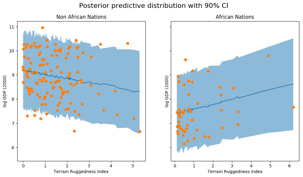
我们观察到,模型的输出和 90% 置信区间解释了我们在实践中观察到的大部分数据点。进行这样的后验预测检查通常是个好主意,以查看我们的模型是否给出了有效的预测。
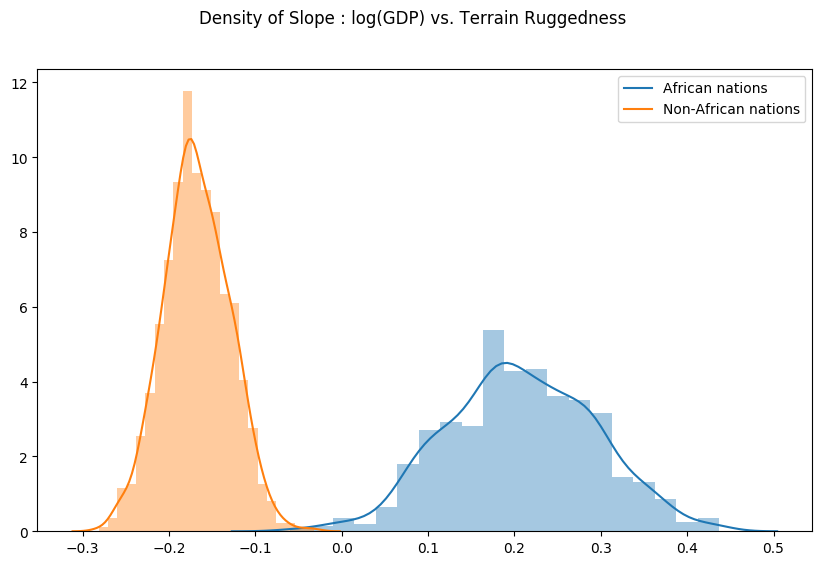
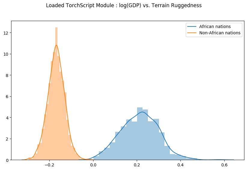
最后,让我们重新审视我们之前的问题,即地形崎岖度与 GDP 之间的关系对于模型参数估计中的任何不确定性有多稳健。为此,我们绘制了非洲内部和外部国家对数 GDP 随地形崎岖度变化的斜率分布。如下图所示,非洲国家的概率质量主要集中在正值区域,而其他国家则相反,这进一步证实了原始假设。
[18]:
weight = samples["linear.weight"]
weight = weight.reshape(weight.shape[0], 3)
gamma_within_africa = weight[:, 1] + weight[:, 2]
gamma_outside_africa = weight[:, 1]
fig = plt.figure(figsize=(10, 6))
sns.distplot(gamma_within_africa, kde_kws={"label": "African nations"},)
sns.distplot(gamma_outside_africa, kde_kws={"label": "Non-African nations"})
fig.suptitle("Density of Slope : log(GDP) vs. Terrain Ruggedness");
通过 TorchScript 进行模型服务
最后,请注意,model、guide 和 Predictive 实用类都是 torch.nn.Module 实例,并且可以序列化为 TorchScript。
在这里,我们展示如何将 Pyro 模型部署为 torch.jit.ModuleScript,它可以作为 C++ 程序独立运行,无需 Python 运行时。
为此,我们将使用 Pyro 的 效果处理库 (effect handling library) 重写我们自己的简单版 Predictive 实用类。这利用了:
tracepoutine 来捕获运行 model/guide 代码的执行轨迹。replaypoutine 来将模型中的 sites 条件化为从 guide trace 中采样的值。
[19]:
from collections import defaultdict
from pyro import poutine
from pyro.poutine.util import prune_subsample_sites
import warnings


class Predict(torch.nn.Module):
    def __init__(self, model, guide):
        super().__init__()
        self.model = model
        self.guide = guide

    def forward(self, *args, **kwargs):
        samples = {}
        guide_trace = poutine.trace(self.guide).get_trace(*args, **kwargs)
        model_trace = poutine.trace(poutine.replay(self.model, guide_trace)).get_trace(*args, **kwargs)
        for site in prune_subsample_sites(model_trace).stochastic_nodes:
            samples[site] = model_trace.nodes[site]['value']
        return tuple(v for _, v in sorted(samples.items()))

predict_fn = Predict(model, guide)
predict_module = torch.jit.trace_module(predict_fn, {"forward": (x_data,)}, check_trace=False)
我们使用 torch.jit.trace_module 追踪该模块的 forward 方法,并使用 torch.jit.save 保存。这个保存的模型 reg_predict.pt 可以使用 PyTorch 的 C++ API 通过 torch::jit::load(filename) 加载,或者像我们下面这样使用 Python API 加载。
[20]:
torch.jit.save(predict_module, '/tmp/reg_predict.pt')
pred_loaded = torch.jit.load('/tmp/reg_predict.pt')
pred_loaded(x_data)
[20]:
(tensor([9.2165]),
 tensor([[-1.6612, -0.1498,  0.4282]]),
 tensor([ 7.5951,  8.2473,  9.3864,  9.2590,  9.0540,  9.3915,  8.6764,  9.3775,
          9.5473,  9.6144, 10.3521,  8.5452,  5.4008,  8.4601,  9.6219,  9.7774,
          7.1958,  7.2581,  8.9159,  9.0875,  8.3730,  8.7903,  9.3167,  8.8155,
          7.4433,  9.9981,  8.6909,  9.2915, 10.1376,  7.7618, 10.1916,  7.4754,
          6.3473,  7.7584,  9.1307,  6.0794,  8.5641,  7.8487,  9.2828,  9.0763,
          7.9250, 10.9226,  8.0005, 10.1799,  5.3611,  8.1174,  8.0585,  8.5098,
          6.8656,  8.6765,  7.8925,  9.5233, 10.1269, 10.2661,  7.8883,  8.9194,
         10.2866,  7.0821,  8.2370,  8.3087,  7.8408,  8.4891,  8.0107,  7.6815,
          8.7497,  9.3551,  9.9687, 10.4804,  8.5176,  7.1679, 10.8805,  7.4919,
          8.7088,  9.2417,  9.2360,  9.7907,  8.4934,  7.8897,  9.5338,  9.6572,
          9.6604,  9.9855,  6.7415,  8.1721, 10.0646, 10.0817,  8.4503,  9.2588,
          8.4489,  7.7516,  6.8496,  9.2208,  8.9852, 10.6585,  9.4218,  9.1290,
          9.5631,  9.7422, 10.2814,  7.2624,  9.6727,  8.9743,  6.9666,  9.5856,
          9.2518,  8.4207,  8.6988,  9.1914,  7.8161,  9.8446,  6.5528,  8.5518,
          6.7168,  7.0694,  8.9211,  8.5311,  8.4545, 10.8346,  7.8768,  9.2537,
          9.0776,  9.4698,  7.9611,  9.2177,  8.0880,  8.5090,  9.2262,  8.9242,
          9.3966,  7.5051,  9.1014,  8.9601,  7.7225,  8.7569,  8.5847,  8.8465,
          9.7494,  8.8587,  6.5624,  6.9372,  9.9806, 10.1259,  9.1864,  7.5758,
          9.8258,  8.6375,  7.6954,  8.9718,  7.0985,  8.6360,  8.5951,  8.9163,
          8.4661,  8.4551, 10.6844,  7.5948,  8.7568,  9.5296,  8.9530,  7.1214,
          9.1401,  8.4992,  8.9115, 10.9739,  8.1593, 10.1162,  9.7072,  7.8641,
          8.8606,  7.5935]),
 tensor(0.9631))
让我们通过从加载的模块生成样本并重新生成之前的图来检查我们的 Predict 模块是否确实正确序列化了。
[21]:
weight = []
for _ in range(800):
    # index = 1 corresponds to "linear.weight"
    weight.append(pred_loaded(x_data)[1])
weight = torch.stack(weight).detach()
weight = weight.reshape(weight.shape[0], 3)
gamma_within_africa = weight[:, 1] + weight[:, 2]
gamma_outside_africa = weight[:, 1]
fig = plt.figure(figsize=(10, 6))
sns.distplot(gamma_within_africa, kde_kws={"label": "African nations"},)
sns.distplot(gamma_outside_africa, kde_kws={"label": "Non-African nations"})
fig.suptitle("Loaded TorchScript Module : log(GDP) vs. Terrain Ruggedness");
在下一节中,我们将探讨如何编写用于变分推断的 guide,并将其结果与通过 HMC 进行的推断结果进行比较。
参考文献
McElreath, D., Statistical Rethinking, Chapter 7, 2016
Nunn, N. & Puga, D., Ruggedness: The blessing of bad geography in Africa”, Review of Economics and Statistics 94(1), Feb. 2012