提升黑箱变分推断

简介

本教程演示了如何在 Pyro 中实现提升黑箱变分推断 [1]。在提升变分推断 [2] 中，我们使用迭代选择的密度混合来近似目标分布。当普通变分推断提供的单一密度无法充分近似目标密度时，提升变分推断提供了一种获得更复杂近似的简单方法。我们将展示如何将其实现为 Pyro SVI 的一个相对简单的扩展。

目录

• 理论背景

  • 变分推断

  • 提升黑箱变分推断

• Pyro 中的 BBBVI

  • 模型

  • 引导分布

  • RELBO

  • 近似

  • 贪婪算法

理论背景

变分推断

对于普通变分推断的介绍，我们建议阅读 Pyro 中的 SVI 教程以及这篇优秀的综述 [3]。

简而言之，变分推断允许我们找到难以进行解析计算的概率密度的近似。例如，可能存在观测变量 \(\textbf{x}\)、潜变量 \(\textbf{z}\) 和联合分布 \(p(\textbf{x}, \textbf{z})\)。然后可以使用变分推断来近似 \(p(\textbf{z}|\textbf{x})\)。为此，首先选择一组易于处理的密度（即一个变分族），然后尝试找到该族中与目标分布 \(p(\textbf{z}|\textbf{x})\) 最接近的元素。这个近似密度是通过最大化证据下界 (ELBO) 找到的

\[\mathbb{E}_q[\log p(\mathbf{x}, \mathbf{z})] - \mathbb{E}_q[\log q(\mathbf{z})]\]

其中 \(q(\mathbf{z})\) 是近似密度。

提升黑箱变分推断

在提升黑箱变分推断 (BBBVI) 中，我们使用来自变分族的密度混合来近似目标密度

\[q^t(\mathbf{z}) = \sum_{i=1}^t \gamma_i s_i(\mathbf{z})\]

\[\text{其中} \sum_{i=1}^t \gamma_i =1\]

且 \(s_t(\mathbf{z})\) 是变分族的元素。

近似的组成部分通过贪婪地最大化所谓的残差 ELBO (RELBO) 来选择，最大化对象是下一个组成部分 \(s_{t+1}(\mathbf{z})\)

\[\mathbb{E}_s[\log p(\mathbf{x},\mathbf{z})] - \lambda \mathbb{E}_s[\log s(\mathbf{z})] - \mathbb{E}_s[\log q^t(\mathbf{z})]\]

其中前两项与 ELBO 中的相同，最后一项是下一个组成部分 \(s_{t+1}(\mathbf{z})\) 和当前近似 \(q^t(\mathbf{z})\) 之间的交叉熵。

这被称为黑箱变分推断（Variational Inference），因为这种优化无需针对所使用的变分族进行定制。通过将 \(\lambda\)（熵项的正则化因子）设置为 1，可以使用标准的 SVI 方法来计算 \(\mathbb{E}_s[\log p(\mathbf{x}, \mathbf{z})] - \lambda \mathbb{E}_s[\log s(\mathbf{z})]\)。关于如何计算 \(- \mathbb{E}_s[\log q^t(\mathbf{z})]\) 项的解释，请参阅下面的RELBO 实现章节。重要的是，我们无需对正在使用的变分族做任何额外假设来确保该算法收敛。

在文献 [1] 中，提出了多种寻找混合权重 \(\gamma_t\) 的方法，从基于迭代的固定步长到求解最小化 RELBO 的优化问题。在这里，我们使用了固定步长方法。有关 Boosting 黑箱变分推断背后理论的更多详情，请参阅文献 [1]。

Pyro 中的 BBBVI

要在 Pyro 中实现 Boosting 黑箱变分推断，我们需要考虑以下几点： 1. 近似分量 \(s_{t}(\mathbf{z})\) (guides)。 2. RELBO。 3. 近似本身 \(q^t(\mathbf{z})\)。 4. 使用 Pyro 的 SVI 来寻找近似的新分量。

我们将通过一个简单的例子来阐述这些要点：近似双峰后验。

import os
from collections import defaultdict
from functools import partial

import numpy as np
import pyro
import pyro.distributions as dist
import scipy.stats
import torch
import torch.distributions.constraints as constraints
from matplotlib import pyplot
from pyro.infer import SVI, Trace_ELBO
from pyro.optim import Adam
from pyro.poutine import block, replay, trace

模型

当我们想要近似多峰分布时，Boosting BBVI 特别有用。在本教程中，我们将考虑以下模型

\[\mathbf{z} \sim \mathcal{N}(0,5)\]

\[\mathbf{x} \sim \mathcal{N}(\mathbf{z}^2, 0.1)\]

给定一组 iid. 观测值 \(\text{data} ~ \mathcal{N}(4, 0.1)\)，我们因此期望 \(p(\mathbf{z}|\mathbf{x})\) 是一个双峰分布，其峰值位于 \(-2\) 和 \(2\) 附近。

在 Pyro 中，这个模型形式如下

def model(data):
    prior_loc = torch.tensor([0.])
    prior_scale = torch.tensor([5.])
    z = pyro.sample('z', dist.Normal(prior_loc, prior_scale))
    scale = torch.tensor([0.1])

    with pyro.plate('data', len(data)):
        pyro.sample('x', dist.Normal(z*z, scale), obs=data)

Guide

接下来，我们指定 guide，在我们的例子中，guide 将构成我们混合分布的分量。回想一下，在 Pyro 中，guide 需要接受与模型相同的参数，这就是为什么我们的 guide 函数也将数据作为输入的原因。

我们还需要确保模型中的每个 pyro.sample() 语句在 guide 中都有对应的 pyro.sample() 语句。在我们的例子中，我们在模型和 guide 中都包含了 z。

与常规 SVI 不同，我们的 guide 接受一个额外参数：index。拥有这个参数使我们能够在贪婪算法的每次迭代中轻松创建新的 guide。具体来说，我们利用 functools 库中的 partial() 来创建只接受 data 作为参数的 guide。语句 partial(guide, index=t) 创建了一个 guide，它将只接受 data 作为输入，并且具有可训练参数 scale_t 和 loc_t。

选择我们的变分分布是由 \(loc_t\) 和 \(scale_t\) 参数化的正态分布，我们得到以下 guide

def guide(data, index):
    scale_q = pyro.param('scale_{}'.format(index), torch.tensor([1.0]), constraints.positive)
    loc_q = pyro.param('loc_{}'.format(index), torch.tensor([0.0]))
    pyro.sample("z", dist.Normal(loc_q, scale_q))

RELBO

我们将 RELBO 实现为一个函数，该函数可以传递给 Pyro 的 SVI 类来代替 ELBO，从而寻找近似分量 \(s_t(z)\)。回想一下，RELBO 形式如下

\[\mathbb{E}_s[\log p(\mathbf{x},\mathbf{z})] - \lambda \mathbb{E}_s[\log s(\mathbf{z})] - \mathbb{E}_s[\log q^t(\mathbf{z})]\]

方便的是，这与常规 ELBO 非常相似，这使得我们能够重用 Pyro 现有的 ELBO。具体来说，我们计算

\[\mathbb{E}_s[\log p(x,z)] - \lambda \mathbb{E}_s[\log s]\]

使用 Pyro 的 Trace_ELBO，然后计算

\[- \mathbb{E}_s[\log q^t]\]

使用 Poutine。有关其工作原理的更多信息，我们建议您参阅 Pyro 关于Poutine 的教程和自定义 SVI 目标函数的教程。

def relbo(model, guide, *args, **kwargs):
    approximation = kwargs.pop('approximation')

    # We first compute the elbo, but record a guide trace for use below.
    traced_guide = trace(guide)
    elbo = pyro.infer.Trace_ELBO(max_plate_nesting=1)
    loss_fn = elbo.differentiable_loss(model, traced_guide, *args, **kwargs)

    # We do not want to update parameters of previously fitted components
    # and thus block all parameters in the approximation apart from z.
    guide_trace = traced_guide.trace
    replayed_approximation = trace(replay(block(approximation, expose=['z']), guide_trace))
    approximation_trace = replayed_approximation.get_trace(*args, **kwargs)

    relbo = -loss_fn - approximation_trace.log_prob_sum()

    # By convention, the negative (R)ELBO is returned.
    return -relbo

近似

我们的近似 \(q^t(z) = \sum_{i=1}^t \gamma_i s_i(z)\) 的实现包含一个分量列表（即来自贪婪选择步骤的 guide）和一个包含这些分量混合权重的列表。要从近似中采样，我们因此首先根据混合权重采样一个分量。第二步，我们从对应的分量中抽取一个样本。

与 guide 类似，我们使用 partial(approximation, components=components, weights=weights) 来获取一个近似函数，其函数签名与模型相同。

def approximation(data, components, weights):
    assignment = pyro.sample('assignment', dist.Categorical(weights))
    result = components[assignment](data)
    return result

贪婪算法

我们现在拥有实现贪婪算法所需的所有部分。首先，我们初始化近似

initial_approximation = partial(guide, index=0)
components = [initial_approximation]
weights = torch.tensor([1.])
wrapped_approximation = partial(approximation, components=components, weights=weights)

然后我们通过在每一步最大化 RELBO 来迭代地寻找近似的 \(T\) 个分量

# clear the param store in case we're in a REPL
pyro.clear_param_store()

# Sample observations from a Normal distribution with loc 4 and scale 0.1
n = torch.distributions.Normal(torch.tensor([4.0]), torch.tensor([0.1]))
data = n.sample((100,))

#T=2
smoke_test = ('CI' in os.environ)
n_steps = 2 if smoke_test else 12000
pyro.set_rng_seed(2)
n_iterations = 2
locs = [0]
scales = [0]
for t in range(1, n_iterations + 1):

    # Create guide that only takes data as argument
    wrapped_guide = partial(guide, index=t)
    losses = []

    adam_params = {"lr": 0.01, "betas": (0.90, 0.999)}
    optimizer = Adam(adam_params)

    # Pass our custom RELBO to SVI as the loss function.
    svi = SVI(model, wrapped_guide, optimizer, loss=relbo)
    for step in range(n_steps):
        # Pass the existing approximation to SVI.
        loss = svi.step(data, approximation=wrapped_approximation)
        losses.append(loss)

        if step % 100 == 0:
            print('.', end=' ')

    # Update the list of approximation components.
    components.append(wrapped_guide)

    # Set new mixture weight.
    new_weight = 2 / (t + 1)

    # In this specific case, we set the mixture weight of the second component to 0.5.
    if t == 2:
        new_weight = 0.5
    weights = weights * (1-new_weight)
    weights = torch.cat((weights, torch.tensor([new_weight])))

    # Update the approximation
    wrapped_approximation = partial(approximation, components=components, weights=weights)

    print('Parameters of component {}:'.format(t))
    scale = pyro.param("scale_{}".format(t)).item()
    scales.append(scale)
    loc = pyro.param("loc_{}".format(t)).item()
    locs.append(loc)
    print('loc = {}'.format(loc))
    print('scale = {}'.format(scale))

. . . . . . . . . . . . . . . . . . . . . . . . . . . . . . . . . . . . . . . . . . . . . . . . . . . . . . . . . . . . . . . . . . . . . . . . . . . . . . . . . . . . . . . . . . . . . . . . . . . . . . . . . . . . . . . . . . . . . . . . Parameters of component 1:
loc = -2.0068717002868652
scale = 0.01799079217016697
. . . . . . . . . . . . . . . . . . . . . . . . . . . . . . . . . . . . . . . . . . . . . . . . . . . . . . . . . . . . . . . . . . . . . . . . . . . . . . . . . . . . . . . . . . . . . . . . . . . . . . . . . . . . . . . . . . . . . . . . Parameters of component 2:
loc = 2.0046799182891846
scale = 0.06008879840373993

# Plot the resulting approximation
X = np.arange(-10, 10, 0.1)
pyplot.figure(figsize=(10, 4), dpi=100).set_facecolor('white')
total_approximation = np.zeros(X.shape)
for i in range(1, n_iterations + 1):
    Y = weights[i].item() * scipy.stats.norm.pdf((X - locs[i]) / scales[i])
    pyplot.plot(X, Y)
    total_approximation += Y
pyplot.plot(X, total_approximation)
pyplot.plot(data.data.numpy(), np.zeros(len(data)), 'k*')
pyplot.title('Approximation of posterior over z')
pyplot.ylabel('probability density')
pyplot.show()

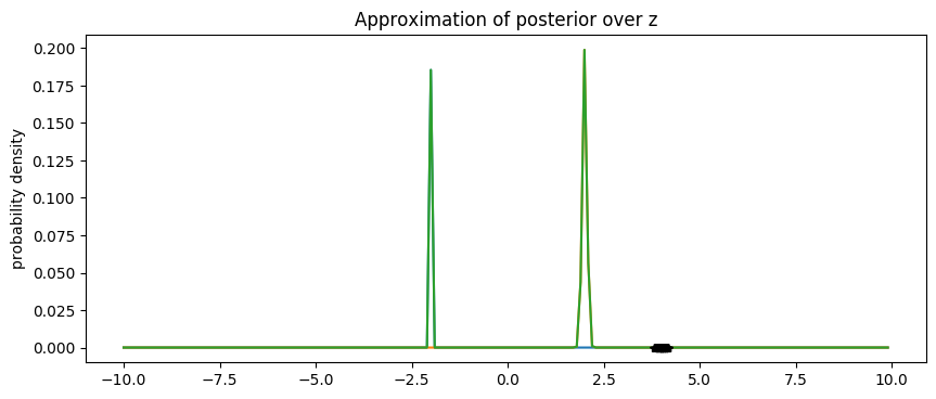
我们看到，Boosting BBVI 成功地近似了峰值位于 -2 和 +2 附近的双峰后验分布。

完整实现

将所有部分组合在一起，我们就得到了 Boosting 黑箱变分推断的完整实现

import os
from collections import defaultdict
from functools import partial

import numpy as np
import pyro
import pyro.distributions as dist
import scipy.stats
import torch
import torch.distributions.constraints as constraints
from matplotlib import pyplot
from pyro.infer import SVI, Trace_ELBO
from pyro.optim import Adam
from pyro.poutine import block, replay, trace

# this is for running the notebook in our testing framework
n_steps = 2 if smoke_test else 12000
pyro.set_rng_seed(2)

# clear the param store in case we're in a REPL
pyro.clear_param_store()

# Sample observations from a Normal distribution with loc 4 and scale 0.1
n = torch.distributions.Normal(torch.tensor([4.0]), torch.tensor([0.1]))
data = n.sample((100,))


def guide(data, index):
    scale_q = pyro.param('scale_{}'.format(index), torch.tensor([1.0]), constraints.positive)
    loc_q = pyro.param('loc_{}'.format(index), torch.tensor([0.0]))
    pyro.sample("z", dist.Normal(loc_q, scale_q))


def model(data):
    prior_loc = torch.tensor([0.])
    prior_scale = torch.tensor([5.])
    z = pyro.sample('z', dist.Normal(prior_loc, prior_scale))
    scale = torch.tensor([0.1])

    with pyro.plate('data', len(data)):
        pyro.sample('x', dist.Normal(z*z, scale), obs=data)


def relbo(model, guide, *args, **kwargs):
    approximation = kwargs.pop('approximation')

    # We first compute the elbo, but record a guide trace for use below.
    traced_guide = trace(guide)
    elbo = pyro.infer.Trace_ELBO(max_plate_nesting=1)
    loss_fn = elbo.differentiable_loss(model, traced_guide, *args, **kwargs)

    # We do not want to update parameters of previously fitted components
    # and thus block all parameters in the approximation apart from z.
    guide_trace = traced_guide.trace
    replayed_approximation = trace(replay(block(approximation, expose=['z']), guide_trace))
    approximation_trace = replayed_approximation.get_trace(*args, **kwargs)

    relbo = -loss_fn - approximation_trace.log_prob_sum()

    # By convention, the negative (R)ELBO is returned.
    return -relbo


def approximation(data, components, weights):
    assignment = pyro.sample('assignment', dist.Categorical(weights))
    result = components[assignment](data)
    return result


def boosting_bbvi():
    # T=2
    n_iterations = 2
    initial_approximation = partial(guide, index=0)
    components = [initial_approximation]
    weights = torch.tensor([1.])
    wrapped_approximation = partial(approximation, components=components, weights=weights)

    locs = [0]
    scales = [0]

    for t in range(1, n_iterations + 1):

        # Create guide that only takes data as argument
        wrapped_guide = partial(guide, index=t)
        losses = []

        adam_params = {"lr": 0.01, "betas": (0.90, 0.999)}
        optimizer = Adam(adam_params)

        # Pass our custom RELBO to SVI as the loss function.
        svi = SVI(model, wrapped_guide, optimizer, loss=relbo)
        for step in range(n_steps):
            # Pass the existing approximation to SVI.
            loss = svi.step(data, approximation=wrapped_approximation)
            losses.append(loss)

            if step % 100 == 0:
                print('.', end=' ')

        # Update the list of approximation components.
        components.append(wrapped_guide)

        # Set new mixture weight.
        new_weight = 2 / (t + 1)

        # In this specific case, we set the mixture weight of the second component to 0.5.
        if t == 2:
            new_weight = 0.5
        weights = weights * (1-new_weight)
        weights = torch.cat((weights, torch.tensor([new_weight])))

        # Update the approximation
        wrapped_approximation = partial(approximation, components=components, weights=weights)

        print('Parameters of component {}:'.format(t))
        scale = pyro.param("scale_{}".format(t)).item()
        scales.append(scale)
        loc = pyro.param("loc_{}".format(t)).item()
        locs.append(loc)
        print('loc = {}'.format(loc))
        print('scale = {}'.format(scale))


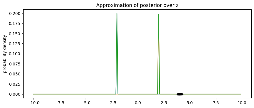
    # Plot the resulting approximation
    X = np.arange(-10, 10, 0.1)
    pyplot.figure(figsize=(10, 4), dpi=100).set_facecolor('white')
    total_approximation = np.zeros(X.shape)
    for i in range(1, n_iterations + 1):
        Y = weights[i].item() * scipy.stats.norm.pdf((X - locs[i]) / scales[i])
        pyplot.plot(X, Y)
        total_approximation += Y
    pyplot.plot(X, total_approximation)
    pyplot.plot(data.data.numpy(), np.zeros(len(data)), 'k*')
    pyplot.title('Approximation of posterior over z')
    pyplot.ylabel('probability density')
    pyplot.show()

if __name__ == '__main__':
    boosting_bbvi()

. . . . . . . . . . . . . . . . . . . . . . . . . . . . . . . . . . . . . . . . . . . . . . . . . . . . . . . . . . . . . . . . . . . . . . . . . . . . . . . . . . . . . . . . . . . . . . . . . . . . . . . . . . . . . . . . . . . . . . . . Parameters of component 1:
loc = -1.9996534585952759
scale = 0.016739774495363235
. . . . . . . . . . . . . . . . . . . . . . . . . . . . . . . . . . . . . . . . . . . . . . . . . . . . . . . . . . . . . . . . . . . . . . . . . . . . . . . . . . . . . . . . . . . . . . . . . . . . . . . . . . . . . . . . . . . . . . . . Parameters of component 2:
loc = 1.998241901397705
scale = 0.01308442372828722

参考文献

[1] Locatello, Francesco, et al. “Boosting 黑箱变分推断（Boosting black box variational inference）.” Advances in Neural Information Processing Systems. 2018.

[2] Ranganath, Rajesh, Sean Gerrish, and David Blei. “黑箱变分推断（Black box variational inference）.” Artificial Intelligence and Statistics. 2014.

[3] Blei, David M., Alp Kucukelbir, and Jon D. McAuliffe. “变分推断：写给统计学家的综述（Variational inference: A review for statisticians）.” Journal of the American statistical Association 112.518 (2017): 859-877.