预测 III: 分层模型
本教程介绍如何使用 pyro.contrib.forecast 模块进行分层多元时间序列建模。本教程假设读者已熟悉 SVI、张量形状 和 单变量预测。
另请参阅
总结
分层预测与 Pyro 中的其他分层建模类似。
要在 Pyro 中创建分层模型,请使用 plate 上下文管理器。
要在训练期间对数据进行子采样,请将
create_plates()回调函数传递给 Forecaster。您可以对时间序列进行子采样,但不能对
time_plate进行子采样。
[1]:
import math
import torch
import pyro
import pyro.distributions as dist
import pyro.poutine as poutine
from pyro.contrib.examples.bart import load_bart_od
from pyro.contrib.forecast import ForecastingModel, Forecaster, eval_crps
from pyro.infer.reparam import LocScaleReparam, SymmetricStableReparam
from pyro.ops.tensor_utils import periodic_repeat
from pyro.ops.stats import quantile
import matplotlib.pyplot as plt

%matplotlib inline
assert pyro.__version__.startswith('1.9.1')
pyro.set_rng_seed(20200305)
我们再次来看 BART 列车 乘客量数据集
[2]:
dataset = load_bart_od()
print(dataset.keys())
print(dataset["counts"].shape)
print(" ".join(dataset["stations"]))
dict_keys(['stations', 'start_date', 'counts'])
torch.Size([78888, 50, 50])
12TH 16TH 19TH 24TH ANTC ASHB BALB BAYF BERY CAST CIVC COLM COLS CONC DALY DBRK DELN DUBL EMBR FRMT FTVL GLEN HAYW LAFY LAKE MCAR MLBR MLPT MONT NBRK NCON OAKL ORIN PCTR PHIL PITT PLZA POWL RICH ROCK SANL SBRN SFIA SHAY SSAN UCTY WARM WCRK WDUB WOAK
多元时间序列
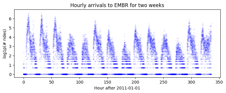
我们首先对来自其他 50 个车站到达 Embarcadero 站的乘客量进行建模。请注意,这是九年的每小时数据,因此数据集相当长。
[3]:
T, O, D = dataset["counts"].shape
data = dataset["counts"][:, :, dataset["stations"].index("EMBR")].log1p()
print(data.shape)
plt.figure(figsize=(9, 3))
plt.plot(data[-24 * 7 * 2:], 'b.', alpha=0.1, markeredgewidth=0)
plt.title("Hourly arrivals to EMBR for two weeks")
plt.ylabel("log1p(# rides)")
plt.xlabel("Hour after 2011-01-01");
torch.Size([78888, 50])
我们尝试一个包含序列本地水平 + 序列本地季节性的双分量模型。
[4]:
class Model1(ForecastingModel):
    def model(self, zero_data, covariates):
        duration, data_dim = zero_data.shape

        # Let's model each time series as a Levy stable process, and share process parameters
        # across time series. To do that in Pyro, we'll declare the shared random variables
        # outside of the "origin" plate:
        drift_stability = pyro.sample("drift_stability", dist.Uniform(1, 2))
        drift_scale = pyro.sample("drift_scale", dist.LogNormal(-20, 5))
        with pyro.plate("origin", data_dim, dim=-2):
            # Now inside of the origin plate we sample drift and seasonal components.
            # All the time series inside the "origin" plate are independent,
            # given the drift parameters above.
            with self.time_plate:
                # We combine two different reparameterizers: the inner SymmetricStableReparam
                # is needed for the Stable site, and the outer LocScaleReparam is optional but
                # appears to improve inference.
                with poutine.reparam(config={"drift": LocScaleReparam()}):
                    with poutine.reparam(config={"drift": SymmetricStableReparam()}):
                        drift = pyro.sample("drift",
                                            dist.Stable(drift_stability, 0, drift_scale))

            with pyro.plate("hour_of_week", 24 * 7, dim=-1):
                seasonal = pyro.sample("seasonal", dist.Normal(0, 5))

        # Now outside of the time plate we can perform time-dependent operations like
        # integrating over time. This allows us to create a motion with slow drift.
        seasonal = periodic_repeat(seasonal, duration, dim=-1)
        motion = drift.cumsum(dim=-1)  # A Levy stable motion to model shocks.
        prediction = motion + seasonal

        # Next we do some reshaping. Pyro's forecasting framework assumes all data is
        # multivariate of shape (duration, data_dim), but the above code uses an "origins"
        # plate that is left of the time_plate. Our prediction starts off with shape
        assert prediction.shape[-2:] == (data_dim, duration)
        # We need to swap those dimensions but keep the -2 dimension intact, in case Pyro
        # adds sample dimensions to the left of that.
        prediction = prediction.unsqueeze(-1).transpose(-1, -3)
        assert prediction.shape[-3:] == (1, duration, data_dim), prediction.shape

        # Finally we can construct a noise distribution.
        # We will share parameters across all time series.
        obs_scale = pyro.sample("obs_scale", dist.LogNormal(-5, 5))
        noise_dist = dist.Normal(0, obs_scale.unsqueeze(-1))
        self.predict(noise_dist, prediction)
现在我们将数据分割为训练集和测试集。这是一个更大的数据集,因此我们只使用 90 天的数据进行训练。
[5]:
T2 = data.size(-2)    # end
T1 = T2 - 24 * 7 * 2  # train/test split
T0 = T1 - 24 * 90     # beginning: train on 90 days of data
covariates = torch.zeros(data.size(-2), 0)  # empty covariates
[6]:
%%time
pyro.set_rng_seed(1)
pyro.clear_param_store()
covariates = torch.zeros(len(data), 0)  # empty
forecaster = Forecaster(Model1(), data[T0:T1], covariates[T0:T1],
                        learning_rate=0.1, num_steps=501, log_every=50)
for name, value in forecaster.guide.median().items():
    if value.numel() == 1:
        print("{} = {:0.4g}".format(name, value.item()))
INFO     step    0 loss = 705188
INFO     step   50 loss = 7.7227
INFO     step  100 loss = 3.44737
INFO     step  150 loss = 1.98431
INFO     step  200 loss = 1.48724
INFO     step  250 loss = 1.25238
INFO     step  300 loss = 1.18827
INFO     step  350 loss = 1.12238
INFO     step  400 loss = 1.10252
INFO     step  450 loss = 1.07717
INFO     step  500 loss = 1.05626
drift_stability = 1.997
drift_scale = 3.863e-08
obs_scale = 0.4636
CPU times: user 28.1 s, sys: 4.29 s, total: 32.4 s
Wall time: 31.9 s
[7]:
samples = forecaster(data[T0:T1], covariates[T0:T2], num_samples=100)
samples.clamp_(min=0)  # apply domain knowledge: the samples must be positive
p10, p50, p90 = quantile(samples[:, 0], (0.1, 0.5, 0.9)).squeeze(-1)
crps = eval_crps(samples, data[T1:T2])
print(samples.shape, p10.shape)

fig, axes = plt.subplots(8, 1, figsize=(9, 10), sharex=True)
plt.subplots_adjust(hspace=0)
axes[0].set_title("log1p(# hourly arrivals to EMBR) (CRPS = {:0.3g})".format(crps))
for i, ax in enumerate(axes):
    ax.axvline(78736, color="green", lw=20, alpha=0.2)
    ax.fill_between(torch.arange(T1, T2), p10[:, i], p90[:, i], color="red", alpha=0.3)
    ax.plot(torch.arange(T1, T2), p50[:, i], 'r-', lw=1, label='forecast')
    ax.plot(torch.arange(T1 - 24 * 7, T2),
            data[T1 - 24 * 7: T2, i], 'k-', lw=1, label='truth')
    ax.set_ylabel("from {}".format(dataset["stations"][i]))
ax.set_xlabel("Hour after 2011-01-01")
ax.text(78732, -3, "Christmas", color="green", horizontalalignment="center")
ax.set_xlim(T1 - 24 * 7, T2)
axes[0].legend(loc="best");
torch.Size([100, 1, 336, 50]) torch.Size([336, 50])
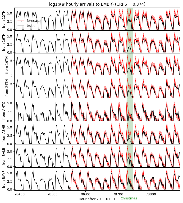
注意圣诞节假期的预测效果较差。这是预料之中的,因为我们只使用 90 天的数据进行训练,并且没有对假期进行建模。为了准确预测假期行为,我们需要使用多年数据进行训练,包括年度季节性分量,并且最好在协变量中包含假期特征。
更深层次的分层模型
接下来我们考虑一个更大的层次结构:所有 50 x 50 = 2500 对车站。
[8]:
data = dataset["counts"].permute(1, 2, 0).unsqueeze(-1).log1p().contiguous()
print(dataset["counts"].shape, data.shape)
torch.Size([78888, 50, 50]) torch.Size([50, 50, 78888, 1])
该模型将有三个层次:起点、终点和时间,每个都建模为一个 plate。我们可以在 plate 上下文的多种组合中创建采样点,从而实现多种共享统计强度的方式。
[9]:
class Model2(ForecastingModel):
    def model(self, zero_data, covariates):
        num_stations, num_stations, duration, one = zero_data.shape

        # We construct plates once so we can reuse them later. We ensure they don't collide by
        # specifying different dim args for each: -3, -2, -1. Note the time_plate is dim=-1.
        origin_plate = pyro.plate("origin", num_stations, dim=-3)
        destin_plate = pyro.plate("destin", num_stations, dim=-2)
        hour_of_week_plate = pyro.plate("hour_of_week", 24 * 7, dim=-1)

        # Let's model the time-dependent part with only O(num_stations * duration) many
        # parameters, rather than the full possible O(num_stations ** 2 * duration) data size.
        drift_stability = pyro.sample("drift_stability", dist.Uniform(1, 2))
        drift_scale = pyro.sample("drift_scale", dist.LogNormal(-20, 5))
        with origin_plate:
            with hour_of_week_plate:
                origin_seasonal = pyro.sample("origin_seasonal", dist.Normal(0, 5))
        with destin_plate:
            with hour_of_week_plate:
                destin_seasonal = pyro.sample("destin_seasonal", dist.Normal(0, 5))
            with self.time_plate:
                with poutine.reparam(config={"drift": LocScaleReparam()}):
                    with poutine.reparam(config={"drift": SymmetricStableReparam()}):
                        drift = pyro.sample("drift",
                                            dist.Stable(drift_stability, 0, drift_scale))
        # Additionally we can model a static pairwise station->station affinity, which e.g.
        # can compensate for the fact that people tend not to travel from a station to itself.
        with origin_plate, destin_plate:
            pairwise = pyro.sample("pairwise", dist.Normal(0, 1))

        # Outside of the time plate we can now form the prediction.
        seasonal = origin_seasonal + destin_seasonal  # Note this broadcasts.
        seasonal = periodic_repeat(seasonal, duration, dim=-1)
        motion = drift.cumsum(dim=-1)  # A Levy stable motion to model shocks.
        prediction = motion + seasonal + pairwise

        # We will decompose the noise scale parameter into
        # an origin-local and a destination-local component.
        with origin_plate:
            origin_scale = pyro.sample("origin_scale", dist.LogNormal(-5, 5))
        with destin_plate:
            destin_scale = pyro.sample("destin_scale", dist.LogNormal(-5, 5))
        scale = origin_scale + destin_scale

        # At this point our prediction and scale have shape (50, 50, duration) and (50, 50, 1)
        # respectively, but we want them to have shape (50, 50, duration, 1) to satisfy the
        # Forecaster requirements.
        scale = scale.unsqueeze(-1)
        prediction = prediction.unsqueeze(-1)

        # Finally we construct a noise distribution and call the .predict() method.
        # Note that predict must be called inside the origin and destination plates.
        noise_dist = dist.Normal(0, scale)
        with origin_plate, destin_plate:
            self.predict(noise_dist, prediction)
[10]:
%%time
pyro.set_rng_seed(1)
pyro.clear_param_store()
covariates = torch.zeros(data.size(-2), 0)  # empty
forecaster = Forecaster(Model2(), data[..., T0:T1, :], covariates[T0:T1],
                        learning_rate=0.1, learning_rate_decay=1, num_steps=501, log_every=50)
for name, value in forecaster.guide.median().items():
    if value.numel() == 1:
        print("{} = {:0.4g}".format(name, value.item()))
INFO     step    0 loss = 4.83016e+10
INFO     step   50 loss = 133310
INFO     step  100 loss = 2.26326
INFO     step  150 loss = 0.879302
INFO     step  200 loss = 0.948082
INFO     step  250 loss = 0.897158
INFO     step  300 loss = 1.43375
INFO     step  350 loss = 0.700097
INFO     step  400 loss = 0.693259
INFO     step  450 loss = 0.691785
INFO     step  500 loss = 0.695014
drift_stability = 1.593
drift_scale = 6.594e-07
CPU times: user 2min 9s, sys: 54.6 s, total: 3min 3s
Wall time: 3min 4s
现在我们可以对每个起点-终点-时间三元组的完整联合样本进行前向预测。forecast(...) 的输出形状将为 (num_samples, num_stations, num_stations, duration, 1)。末尾的 1 仅表示我们将其建模为一批单变量时间序列(尽管带有分层耦合)。
[11]:
%%time
samples = forecaster(data[..., T0:T1, :], covariates[T0:T2], num_samples=100)
samples.clamp_(min=0)  # apply domain knowledge: the samples must be positive
p10, p50, p90 = quantile(samples[..., 0], (0.1, 0.5, 0.9))
crps = eval_crps(samples, data[..., T1:T2, :])
print(samples.shape, p10.shape)
torch.Size([100, 50, 50, 336, 1]) torch.Size([50, 50, 336])
CPU times: user 21.5 s, sys: 7.95 s, total: 29.4 s
Wall time: 32.4 s
现在我们可以查看任意车站对的预测结果。让我们看看 Antioch,它是新车站中乘客量最少的之一。
[12]:
fig, axes = plt.subplots(8, 1, figsize=(9, 10), sharex=True)
plt.subplots_adjust(hspace=0)
j = dataset["stations"].index("ANTC")
axes[0].set_title("log1p(# hourly arrivals to ANTC) (CRPS = {:0.3g})".format(crps))
for i, ax in enumerate(axes):
    ax.axvline(78736, color="green", lw=20, alpha=0.2)
    ax.fill_between(torch.arange(T1, T2), p10[i, j], p90[i, j], color="red", alpha=0.3)
    ax.plot(torch.arange(T1, T2), p50[i, j], 'r-', lw=1, label='forecast')
    ax.plot(torch.arange(T1 - 24 * 7, T2),
            data[i, j, T1 - 24 * 7: T2, 0], 'k-', lw=1, label='truth')
    ax.set_ylabel("from {}".format(dataset["stations"][i]))
ax.set_xlabel("Hour after 2011-01-01")
ax.text(78732, -0.8, "Christmas", color="green", horizontalalignment="center")
ax.set_xlim(T1 - 24 * 7, T2)
axes[0].legend(loc="best");
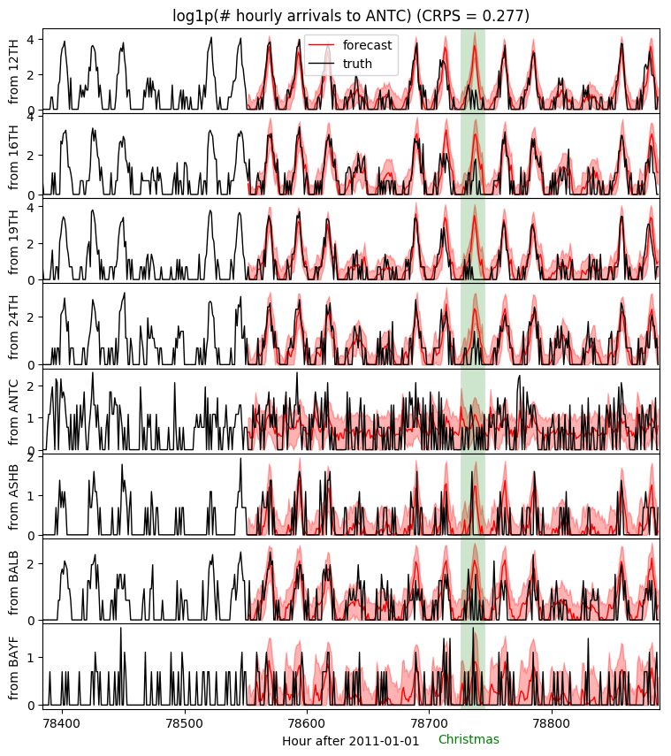
注意,分层模型甚至可以对乘客量非常低的车站对做出准确预测。例如,几乎没有人从 Ashby 站乘坐到 Antioch 站。
子采样
训练高维时间序列数据模型可能很昂贵。然而,由于我们使用随机变分推断进行训练,我们可以对部分数据 plate 进行子采样,以速度换取梯度方差。在我们的 BART 示例中,我们可以对起点和终点都进行子采样(但永远不能对 time_plate 进行子采样)。
要在 Forecaster 中启用子采样(或更一般地说,在任何 Pyro AutoDelta 或 Autonormal guide 中),我们需要定义一个回调函数,该函数在 guide 中创建子采样 plate。此回调函数将命名为 create_plates()。它将输入与模型相同的 (zero_data, covariates) 参数(或更一般地说,相同的 (*args, **kwargs)),并返回一个 plate 或 plate 的可迭代对象。
我们定义一个 create_plates() 回调函数,将“origin” plate 和“destin” plate 都子采样到其数据的 20%,从而在每次迭代中仅触及 4% 的数据。
[13]:
def create_plates(zero_data, covariates):
    num_origins, num_destins, duration, one = zero_data.shape
    return [pyro.plate("origin", num_origins, subsample_size=10, dim=-3),
            pyro.plate("destin", num_destins, subsample_size=10, dim=-2)]
现在我们可以像往常一样进行训练。然而,由于梯度估计将具有更高的方差,我们将运行更多迭代。我们将使用相同的学习率,并让 Adam 优化器调整每个参数的学习率。
[14]:
%%time
pyro.set_rng_seed(1)
pyro.clear_param_store()
covariates = torch.zeros(data.size(-2), 0)  # empty
forecaster = Forecaster(Model2(), data[..., T0:T1, :], covariates[T0:T1],
                        create_plates=create_plates,
                        learning_rate=0.1, num_steps=1201, log_every=50)
for name, value in forecaster.guide.median().items():
    if value.numel() == 1:
        print("{} = {:0.4g}".format(name, value.item()))
INFO     step    0 loss = 58519
INFO     step   50 loss = 3.61814e+09
INFO     step  100 loss = 965.526
INFO     step  150 loss = 9000.55
INFO     step  200 loss = 1003.25
INFO     step  250 loss = 31.0245
INFO     step  300 loss = 1.53046
INFO     step  350 loss = 1.22161
INFO     step  400 loss = 0.991503
INFO     step  450 loss = 0.79876
INFO     step  500 loss = 0.83428
INFO     step  550 loss = 0.804639
INFO     step  600 loss = 0.686404
INFO     step  650 loss = 0.803543
INFO     step  700 loss = 0.783584
INFO     step  750 loss = 0.618151
INFO     step  800 loss = 0.772374
INFO     step  850 loss = 0.684863
INFO     step  900 loss = 0.77464
INFO     step  950 loss = 0.862912
INFO     step 1000 loss = 0.74513
INFO     step 1050 loss = 0.756743
INFO     step 1100 loss = 0.772813
INFO     step 1150 loss = 0.68757
INFO     step 1200 loss = 0.778757
drift_stability = 1.502
drift_scale = 4.265e-07
CPU times: user 46.2 s, sys: 7.11 s, total: 53.3 s
Wall time: 52.9 s
尽管我们运行了更多迭代(1201 次而不是 501 次),但每次迭代的成本更低,并且总时间减少了三倍以上,同时精度几乎相同
[15]:
%%time
samples = forecaster(data[..., T0:T1, :], covariates[T0:T2], num_samples=100)
samples.clamp_(min=0)  # apply domain knowledge: the samples must be positive
crps = eval_crps(samples, data[..., T1:T2, :])
print("CRPS = {:0.4g}".format(crps))
CRPS = 0.2792
CPU times: user 14.6 s, sys: 5.77 s, total: 20.4 s
Wall time: 23.1 s
[ ]: