高斯过程隐变量模型¶

高斯过程隐变量模型 (GPLVM) 是一种降维方法，它使用高斯过程学习（可能是）高维数据的低维表示。在高斯过程回归的典型设置中，给定输入 \(X\) 和输出 \(y\)，我们选择一个核函数并学习最优的超参数来描述从 \(X\) 到 \(y\) 的映射。在 GPLVM 中，我们不知道 \(X\)：我们只知道 \(y\)。因此，我们需要学习 \(X\) 以及核超参数。

我们不对 \(X\) 进行最大似然推断。相反，我们为 \(X\) 设置一个高斯先验，并学习近似（高斯）后验 \(q(X|y)\) 的均值和方差。在本教程中，我们将展示如何使用 pyro.contrib.gp 模块来完成此操作。特别是，我们将重现 [2] 中描述的结果。

[1]:

import os
import matplotlib.pyplot as plt
import pandas as pd
import torch
from torch.nn import Parameter

import pyro
import pyro.contrib.gp as gp
import pyro.distributions as dist
import pyro.ops.stats as stats

smoke_test = ('CI' in os.environ)  # ignore; used to check code integrity in the Pyro repo
assert pyro.__version__.startswith('1.9.1')
pyro.set_rng_seed(1)

数据集¶

我们将使用的数据包括从小鼠获得的 48 个基因的单细胞 qPCR 数据（Guo 等人，[1]）。这些数据可在 Open Data Science 存储库获取。数据包含 48 列，每列对应于每个基因的（归一化）测量值。细胞在发育过程中会分化，这些数据是在不同的发育阶段获得的。不同的阶段从 1 细胞阶段标记到 64 细胞阶段。对于 32 细胞阶段，数据进一步区分到 'trophectoderm' (TE) 和 'inner cell mass' (ICM)。ICM 在 64 细胞阶段进一步分化为 'epiblast' (EPI) 和 'primitive endoderm' (PE)。数据集中的每一行都标有这些阶段之一。

[2]:

# license: Copyright (c) 2014, the Open Data Science Initiative
# license: https://www.elsevier.com/legal/elsevier-website-terms-and-conditions
URL = "https://raw.githubusercontent.com/sods/ods/master/datasets/guo_qpcr.csv"

df = pd.read_csv(URL, index_col=0)
print("Data shape: {}\n{}\n".format(df.shape, "-" * 21))
print("Data labels: {}\n{}\n".format(df.index.unique().tolist(), "-" * 86))
print("Show a small subset of the data:")
df.head()

Data shape: (437, 48)
---------------------

Data labels: ['1', '2', '4', '8', '16', '32 TE', '32 ICM', '64 PE', '64 TE', '64 EPI']
--------------------------------------------------------------------------------------

Show a small subset of the data:

[2]:

	Actb	Ahcy	Aqp3	Atp12a	Bmp4	Cdx2	Creb312	Cebpa	Dab2	DppaI	...	Sox2	Sall4	Sox17	Snail	Sox13	Tcfap2a	Tcfap2c	Tcf23	Utf1	Tspan8
1	0.541050	-1.203007	1.030746	1.064808	0.494782	-0.167143	-1.369092	1.083061	0.668057	-1.553758	...	-1.351757	-1.793476	0.783185	-1.408063	-0.031991	-0.351257	-1.078982	0.942981	1.348892	-1.051999
1	0.680832	-1.355306	2.456375	1.234350	0.645494	1.003868	-1.207595	1.208023	0.800388	-1.435306	...	-1.363533	-1.782172	1.532477	-1.361172	-0.501715	1.082362	-0.930112	1.064399	1.469397	-0.996275
1	1.056038	-1.280447	2.046133	1.439795	0.828121	0.983404	-1.460032	1.359447	0.530701	-1.340283	...	-1.296802	-1.567402	3.194157	-1.301777	-0.445219	0.031284	-1.005767	1.211529	1.615421	-0.651393
1	0.732331	-1.326911	2.464234	1.244323	0.654359	0.947023	-1.265609	1.215373	0.765212	-1.431401	...	-1.684100	-1.915556	2.962515	-1.349710	1.875957	1.699892	-1.059458	1.071541	1.476485	-0.699586
1	0.629333	-1.244308	1.316815	1.304162	0.707552	1.429070	-0.895578	-0.007785	0.644606	-1.381937	...	-1.304653	-1.761825	1.265379	-1.320533	-0.609864	0.413826	-0.888624	1.114394	1.519017	-0.798985

5 行 × 48 列

建模¶

首先，我们需要定义输出张量 \(y\)。为了预测所有 \(48\) 个基因的值，我们需要 \(48\) 个高斯过程。因此，\(y\) 所需的形状是 num_GPs x num_data = 48 x 437。

[3]:

data = torch.tensor(df.values, dtype=torch.get_default_dtype())
# we need to transpose data to correct its shape
y = data.t()

现在是最有趣的部分。我们知道观测数据 \(y\) 具有潜在结构：特别是不同的数据点对应于不同的细胞阶段。我们希望我们的 GPLVM 以无监督的方式学习这种结构。原则上，如果我们做好推断工作，我们就应该能够发现这种结构——至少如果我们选择合理的先验。首先，我们必须选择我们的潜在空间 \(X\) 的维度。我们选择 \(dim(X)=2\)，因为我们希望我们的模型能够将“捕获时间”（\(1\)、\(2\)、\(4\)、\(8\)、\(16\)、\(32\) 和 \(64\)）与细胞分支类型（TE、ICM、PE、EPI）分离。接下来，当我们设置 \(X\) 先验的均值时，我们将第一维设置为等于观测到的捕获时间。这将有助于 GPLVM 发现我们感兴趣的结构，并使其更有可能以一种更容易解释的方式与轴对齐。

[4]:

capture_time = y.new_tensor([int(cell_name.split(" ")[0]) for cell_name in df.index.values])
# we scale the time into the interval [0, 1]
time = capture_time.log2() / 6

# we setup the mean of our prior over X
X_prior_mean = torch.zeros(y.size(1), 2)  # shape: 437 x 2
X_prior_mean[:, 0] = time

我们将使用高斯过程推断的稀疏版本来加快训练速度。请记住，我们还需要将 \(X\) 定义为一个 Parameter，以便我们可以为其设置先验和指导（变分分布）。

[5]:

kernel = gp.kernels.RBF(input_dim=2, lengthscale=torch.ones(2))

# we clone here so that we don't change our prior during the course of training
X = Parameter(X_prior_mean.clone())

# we will use SparseGPRegression model with num_inducing=32;
# initial values for Xu are sampled randomly from X_prior_mean
Xu = stats.resample(X_prior_mean.clone(), 32)
gplvm = gp.models.SparseGPRegression(X, y, kernel, Xu, noise=torch.tensor(0.01), jitter=1e-5)

我们将使用 Parameterized 类中的 autoguide() 方法为 \(X\) 设置一个自动 Normal 指导。

[6]:

# we use `.to_event()` to tell Pyro that the prior distribution for X has no batch_shape
gplvm.X = pyro.nn.PyroSample(dist.Normal(X_prior_mean, 0.1).to_event())
gplvm.autoguide("X", dist.Normal)

推断¶

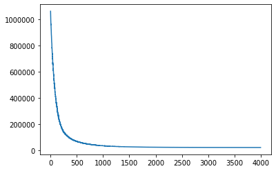
正如高斯过程教程中提到的，我们可以使用辅助函数 gp.util.train 来训练 Pyro GP 模块。默认情况下，此辅助函数使用 Adam 优化器，学习率为 0.01。

[7]:

# note that training is expected to take a minute or so
losses = gp.util.train(gplvm, num_steps=4000)

# let's plot the loss curve after 4000 steps of training
plt.plot(losses)
plt.show()

推断后，近似后验 \(q(X) \sim p(X | y)\) 的均值和标准差将存储在参数 X_loc 和 X_scale 中。要从 \(q(X)\) 中获取样本，我们需要将 gplvm 的 mode 设置为 "guide"。

[8]:

gplvm.mode = "guide"
X = gplvm.X  # draw a sample from the guide of the variable X

结果可视化¶

让我们看看将 GPLVM 应用于我们的数据集得到的结果。

[9]:

plt.figure(figsize=(8, 6))
colors = plt.get_cmap("tab10").colors[::-1]
labels = df.index.unique()

X = gplvm.X_loc.detach().numpy()
for i, label in enumerate(labels):
    X_i = X[df.index == label]
    plt.scatter(X_i[:, 0], X_i[:, 1], c=[colors[i]], label=label)

plt.legend()
plt.xlabel("pseudotime", fontsize=14)
plt.ylabel("branching", fontsize=14)
plt.title("GPLVM on Single-Cell qPCR data", fontsize=16)
plt.show()

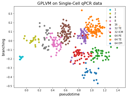
我们可以看到，每个细胞的潜在 \(X\) 的第一维（横轴）与观测到的捕获时间（颜色）很好地对应。另一方面，32 个 TE 细胞和 64 个 TE 细胞聚集在一起。而且，ICM 细胞分化为 PE 和 EPI 的事实也可以从图中观察到！

备注¶

稀疏版本与数据点数量呈线性关系，因此 GPLVM 可用于大型数据集。事实上，在 [2] 中，作者将 GPLVM 应用于包含 68k 个外周血单核细胞的数据集。
高斯过程的大部分强大之处在于由核函数定义的函数先验。我们建议用户尝试不同核函数的组合，以应对不同类型的数据集！例如，如果数据包含周期性，使用周期核可能是有意义的。其他核函数也可以在Pyro GP 文档中找到。

参考文献¶

[1] Resolution of Cell Fate Decisions Revealed by Single-Cell Gene Expression Analysis from Zygote to Blastocyst, Guoji Guo, Mikael Huss, Guo Qing Tong, Chaoyang Wang, Li Li Sun, Neil D. Clarke, Paul Robson

[2] GrandPrix: Scaling up the Bayesian GPLVM for single-cell data, Sumon Ahmed, Magnus Rattray, Alexis Boukouvalas

[3] Bayesian Gaussian Process Latent Variable Model, Michalis K. Titsias, Neil D. Lawrence

[4] A novel approach for resolving differences in single-cell gene expression patterns from zygote to blastocyst, Florian Buettner, Fabian J. Theis