MLE 和 MAP 估计

在这个简短教程中，我们将回顾如何在 Pyro 中进行最大似然估计 (MLE) 和最大后验估计 (MAP)。

import torch
from torch.distributions import constraints
import pyro
import pyro.distributions as dist
from pyro.infer import SVI, Trace_ELBO
import matplotlib.pyplot as plt
%matplotlib inline

我们考虑在之前的教程中介绍的简单“公平硬币”示例。

data = torch.zeros(10)
data[0:6] = 1.0

def original_model(data):
    f = pyro.sample("latent_fairness", dist.Beta(10.0, 10.0))
    with pyro.plate("data", data.size(0)):
        pyro.sample("obs", dist.Bernoulli(f), obs=data)

为了便于比较不同的推断技术，我们构建了一个训练助手

def train(model, guide, lr=0.005, n_steps=201):
    pyro.clear_param_store()
    adam_params = {"lr": lr}
    adam = pyro.optim.Adam(adam_params)
    svi = SVI(model, guide, adam, loss=Trace_ELBO())

    for step in range(n_steps):
        loss = svi.step(data)
        if step % 50 == 0:
            print('[iter {}]  loss: {:.4f}'.format(step, loss))

MLE

我们的模型有一个单一的潜变量 latent_fairness。为了进行最大似然估计，我们只需将潜变量 latent_fairness“降级”为 Pyro 参数。

def model_mle(data):
    # note that we need to include the interval constraint;
    # in original_model() this constraint appears implicitly in
    # the support of the Beta distribution.
    f = pyro.param("latent_fairness", torch.tensor(0.5),
                   constraint=constraints.unit_interval)
    with pyro.plate("data", data.size(0)):
        pyro.sample("obs", dist.Bernoulli(f), obs=data)

我们可以按如下所示渲染我们的模型。

pyro.render_model(model_mle, model_args=(data,), render_distributions=True, render_params=True)

由于我们不再有任何潜变量，我们的 guide 可以是空的

def guide_mle(data):
    pass

让我们看看我们得到什么结果。

train(model_mle, guide_mle)

[iter 0]  loss: 6.9315
[iter 50]  loss: 6.7693
[iter 100]  loss: 6.7333
[iter 150]  loss: 6.7302
[iter 200]  loss: 6.7301

mle_estimate = pyro.param("latent_fairness").item()
print("Our MLE estimate of the latent fairness is {:.3f}".format(mle_estimate))

Our MLE estimate of the latent fairness is 0.600

我们还可以将我们的 MLE 估计与解析 MLE 估计进行比较，后者由以下公式给出：\(\frac{\#Heads}{\#Heads + \#Tails}\)。由于我们将 Heads 编码为 1，将 Tails 编码为 0，我们可以直接将解析 MLE 计算为 data.sum()/data.size(0) 或 data.mean()。

print("The analytical MLE estimate of the latent fairness is {:.3f}".format(
      data.mean()))

The analytical MLE estimate of the latent fairness is 0.600

因此，通过 MLE，我们得到了 latent_fairness 的点估计，它与解析 MLE 估计相匹配。

您可能想知道如何解释我们上述实验中的损失值。损失等同于在 Bernoulli 似然下观测数据的负对数似然 (NLL)。因此，上述过程等同于最小化 NLL。我们在下面确认了这一点。

nll = -dist.Bernoulli(mle_estimate).log_prob(data).sum()
print(f"The negative log likelihood given latent fairness = {mle_estimate:0.3f} is {nll:0.4f} which matches the loss obtained via our training procedure.")

The negative log likelihood given latent fairness = 0.600 is 6.7301 which matches the loss obtained via our training procedure.

MAP

通过最大后验估计，我们也可以得到潜变量的点估计。与 MLE 的区别在于，这些估计会受到先验的正则化。我们可以通过下面的渲染图来理解 MLE 和 MAP 所用模型之间的差异，我们可以看到 latent_fairness 在原始模型中是一个 pyro.sample。

pyro.render_model(original_model, model_args=(data,), render_distributions=True)

要在 Pyro 中进行 MAP，我们使用Delta 分布作为 guide。回想一下，Delta 分布将其所有概率质量集中在一个单一值上。Delta 分布将由一个可学习参数参数化。

def guide_map(data):
    f_map = pyro.param("f_map", torch.tensor(0.5),
                       constraint=constraints.unit_interval)
    pyro.sample("latent_fairness", dist.Delta(f_map))

让我们看看这个结果与 MLE 有何不同。

train(original_model, guide_map)

[iter 0]  loss: 5.6719
[iter 50]  loss: 5.6007
[iter 100]  loss: 5.6004
[iter 150]  loss: 5.6004
[iter 200]  loss: 5.6004

map_estimate = pyro.param("f_map").item()
print("Our MAP estimate of the latent fairness is {:.3f}".format(map_estimate))

Our MAP estimate of the latent fairness is 0.536

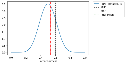
要理解正在发生的事情，请注意我们模型中 latent_fairness 的先验均值为 0.5，因为它是 Beta(10.0, 10.0) 的均值。MLE 估计（忽略先验）给出的结果完全由原始计数（6 个正面和 4 个反面）决定。相比之下，MAP 估计被正则化 towards 先验均值，这就是为什么 MAP 估计在 0.5 和 0.6 之间的某个地方。我们也可以从下面的图中理解这些。实际上，给定 Beta 先验和 Bernoulli 似然，我们也可以解析地计算 MAP 估计。

我们的 Beta 先验由 \(\alpha_{Heads}\) （在我们例子中为 10）和 \(\alpha_{Tails}\) （在我们例子中为 10）参数化。MAP 估计的封闭形式表达式为：\(\frac{\alpha_{Heads} + ~\#Heads}{\alpha_{Heads} + ~\#Heads +~ \alpha_{Tails} + ~\#Tails}\) = \(\frac{10 + 6}{10 + 6 + 10 + 4}\) = \(\frac{16}{30} = 0.5\bar{3}\)

x = torch.linspace(0.0, 1.0, 100)
plt.plot(x, dist.Beta(10, 10).log_prob(x).exp(), label='Prior~Beta(10, 10)')
plt.xlabel("Latent Fairness")
plt.axvline(mle_estimate, color='k', linestyle='--', label='MLE')
plt.axvline(map_estimate, color='r', linestyle='-.', label='MAP')
plt.axvline(0.5, color='g', linestyle=':', label='Prior Mean')
plt.legend(bbox_to_anchor=(1.44,1), borderaxespad=0)

<matplotlib.legend.Legend at 0x7f260a981d90>

使用 AutoGuides 做同样的事情

在上面，我们手动定义了 guides。通常依赖 Pyro 的AutoGuide 机制会更容易。让我们看看如何使用 AutoGuides 进行 MLE 和 MAP 推断。

为了进行 MLE 估计，我们首先使用 `mask(False) <https://docs.pyro.org.cn/en/stable/poutine.html?highlight=mask#pyro.poutine.handlers.mask>`__ 来指示 Pyro 忽略模型中潜变量 latent_fairness 的 log_prob。（注意，我们需要对每个潜变量都这样做。）这样，模型中唯一的非零 log_prob 将来自 Bernoulli 似然，而 ELBO 最大化将等同于似然最大化。

def masked_model(data):
    f = pyro.sample("latent_fairness",
                    dist.Beta(10.0, 10.0).mask(False))
    with pyro.plate("data", data.size(0)):
        pyro.sample("obs", dist.Bernoulli(f), obs=data)

接下来我们定义一个 `AutoDelta <https://docs.pyro.org.cn/en/stable/infer.autoguide.html?highlight=autodelta#autodelta>`__ guide，它学习每个潜变量的点估计（即，我们不学习任何不确定性）

autoguide_mle = pyro.infer.autoguide.AutoDelta(masked_model)
train(masked_model, autoguide_mle)
print("Our MLE estimate of the latent fairness is {:.3f}".format(
      autoguide_mle.median(data)["latent_fairness"].item()))

[iter 0]  loss: 7.0436
[iter 50]  loss: 6.8213
[iter 100]  loss: 6.7467
[iter 150]  loss: 6.7319
[iter 200]  loss: 6.7302
Our MLE estimate of the latent fairness is 0.598

为了进行 MAP 推断，我们再次使用 AutoDelta guide，但这次是在原始模型上，其中 latent_fairness 是一个潜变量

autoguide_map = pyro.infer.autoguide.AutoDelta(original_model)
train(original_model, autoguide_map)
print("Our MAP estimate of the latent fairness is {:.3f}".format(
      autoguide_map.median(data)["latent_fairness"].item()))

[iter 0]  loss: 5.6889
[iter 50]  loss: 5.6005
[iter 100]  loss: 5.6004
[iter 150]  loss: 5.6004
[iter 200]  loss: 5.6004
Our MAP estimate of the latent fairness is 0.536

我们还可以快速验证，如果在原始模型中选择均匀先验，我们的 MAP 估计将与 MLE 估计相同。

def original_model_uniform_prior(data):
    f = pyro.sample("latent_fairness", dist.Uniform(low=0.0, high=1.0))
    with pyro.plate("data", data.size(0)):
        pyro.sample("obs", dist.Bernoulli(f), obs=data)

autoguide_map_uniform_prior = pyro.infer.autoguide.AutoDelta(original_model_uniform_prior)
train(original_model_uniform_prior, autoguide_map_uniform_prior)
print("Our MAP estimate of the latent fairness under the Uniform prior is {:.3f} matching the MLE estimate".format(
      autoguide_map_uniform_prior.median(data)["latent_fairness"].item()))

[iter 0]  loss: 6.7490
[iter 50]  loss: 6.7302
[iter 100]  loss: 6.7301
[iter 150]  loss: 6.7301
[iter 200]  loss: 6.7301
Our MAP estimate of the latent fairness under the Uniform prior is 0.600 matching the MLE estimate