预测 II:状态空间模型
本教程介绍如何使用 pyro.contrib.forecast 模块进行状态空间建模。本教程假设读者已经熟悉 SVI、tensor 形状和单变量预测。
另请参阅
概述
Pyro 的 ForecastingModel 可以结合回归、变分推断和精确推断。
要建模线性高斯动力系统,请使用 GaussianHMM 作为
noise_dist。要建模重尾线性动力系统,请使用带有重尾分布的 LinearHMM。
要实现 LinearHMM 的推断,请使用 LinearHMMReparam 重参数化器。
[1]:
import math
import torch
import pyro
import pyro.distributions as dist
import pyro.poutine as poutine
from pyro.contrib.examples.bart import load_bart_od
from pyro.contrib.forecast import ForecastingModel, Forecaster, eval_crps
from pyro.infer.reparam import LinearHMMReparam, StableReparam, SymmetricStableReparam
from pyro.ops.tensor_utils import periodic_repeat
from pyro.ops.stats import quantile
import matplotlib.pyplot as plt

%matplotlib inline
assert pyro.__version__.startswith('1.9.1')
pyro.set_rng_seed(20200305)
状态空间模型简介
在单变量教程中,我们了解了如何使用变分推断将时间序列建模为回归加上局部水平模型。本教程介绍另一种时间序列建模方法:状态空间模型和精确推断。Pyro 的预测模块允许结合这两种范式,例如使用回归建模季节性(包括缓慢的全局趋势),并使用状态空间模型建模短期局部趋势。
Pyro 实现了一些状态空间模型,但最重要的是 GaussianHMM 分布及其重尾泛化形式 LinearHMM 分布。这两种模型都对具有隐藏状态的线性动力系统进行建模;它们都是多变量的,并且都允许学习所有过程参数。此外,pyro.contrib.timeseries 模块实现了各种多变量高斯过程模型,这些模型可以编译为 GaussianHMM。
Pyro 对 GaussianHMM 的推断使用并行扫描卡尔曼滤波,从而可以快速分析非常长的时间序列。类似地,Pyro 对 LinearHMM 的推断使用完全并行的辅助变量方法将其归约为 GaussianHMM,然后允许进行并行扫描推断。因此,这两种方法都可以并行化长时序分析,即使对于单个单变量时间序列也是如此。
我们再次查看 BART 列车乘客量数据集
[2]:
dataset = load_bart_od()
print(dataset.keys())
print(dataset["counts"].shape)
print(" ".join(dataset["stations"]))
dict_keys(['stations', 'start_date', 'counts'])
torch.Size([78888, 50, 50])
12TH 16TH 19TH 24TH ANTC ASHB BALB BAYF BERY CAST CIVC COLM COLS CONC DALY DBRK DELN DUBL EMBR FRMT FTVL GLEN HAYW LAFY LAKE MCAR MLBR MLPT MONT NBRK NCON OAKL ORIN PCTR PHIL PITT PLZA POWL RICH ROCK SANL SBRN SFIA SHAY SSAN UCTY WARM WCRK WDUB WOAK
[3]:
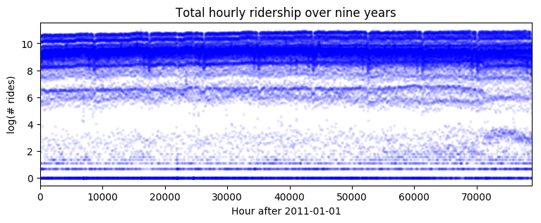
data = dataset["counts"].sum([-1, -2]).unsqueeze(-1).log1p()
print(data.shape)
plt.figure(figsize=(9, 3))
plt.plot(data, 'b.', alpha=0.1, markeredgewidth=0)
plt.title("Total hourly ridership over nine years")
plt.ylabel("log(# rides)")
plt.xlabel("Hour after 2011-01-01")
plt.xlim(0, len(data));
torch.Size([78888, 1])
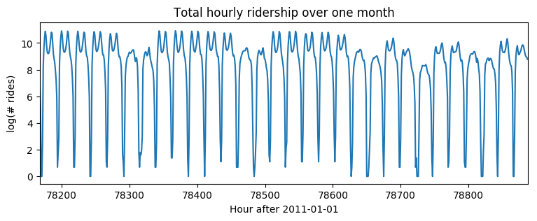
[4]:
plt.figure(figsize=(9, 3))
plt.plot(data)
plt.title("Total hourly ridership over one month")
plt.ylabel("log(# rides)")
plt.xlabel("Hour after 2011-01-01")
plt.xlim(len(data) - 24 * 30, len(data));
GaussianHMM
让我们首先对每小时季节性以及局部线性趋势进行建模,其中我们通过回归建模季节性,通过 GaussianHMM 建模局部线性趋势。这种噪声模型包括一个均值回归隐藏状态(一个 Ornstein-Uhlenbeck 过程)以及高斯观测噪声。
[5]:
T0 = 0                # beginning
T2 = data.size(-2)    # end
T1 = T2 - 24 * 7 * 2  # train/test split
means = data[:T1 // (24 * 7) * 24 * 7].reshape(-1, 24 * 7).mean(0)
[6]:
class Model1(ForecastingModel):
    def model(self, zero_data, covariates):
        duration = zero_data.size(-2)

        # We'll hard-code the periodic part of this model, learning only the local model.
        prediction = periodic_repeat(means, duration, dim=-1).unsqueeze(-1)

        # On top of this mean prediction, we'll learn a linear dynamical system.
        # This requires specifying five pieces of data, on which we will put structured priors.
        init_dist = dist.Normal(0, 10).expand([1]).to_event(1)

        timescale = pyro.sample("timescale", dist.LogNormal(math.log(24), 1))
        # Note timescale is a scalar but we need a 1x1 transition matrix (hidden_dim=1),
        # thus we unsqueeze twice using [..., None, None].
        trans_matrix = torch.exp(-1 / timescale)[..., None, None]
        trans_scale = pyro.sample("trans_scale", dist.LogNormal(-0.5 * math.log(24), 1))
        trans_dist = dist.Normal(0, trans_scale.unsqueeze(-1)).to_event(1)

        # Note the obs_matrix has shape hidden_dim x obs_dim = 1 x 1.
        obs_matrix = torch.tensor([[1.]])
        obs_scale = pyro.sample("obs_scale", dist.LogNormal(-2, 1))
        obs_dist = dist.Normal(0, obs_scale.unsqueeze(-1)).to_event(1)

        noise_dist = dist.GaussianHMM(
            init_dist, trans_matrix, trans_dist, obs_matrix, obs_dist, duration=duration)
        self.predict(noise_dist, prediction)
然后我们可以在多年的数据上训练模型。请注意,由于我们只对时间全局变量进行变分,并精确地积分消除时间局部变量(通过 GaussianHMM),随机梯度方差非常低;这使得我们可以使用较大的学习率和较少的步骤。
[7]:
%%time
pyro.set_rng_seed(1)
pyro.clear_param_store()
covariates = torch.zeros(len(data), 0)  # empty
forecaster = Forecaster(Model1(), data[:T1], covariates[:T1], learning_rate=0.1, num_steps=400)
for name, value in forecaster.guide.median().items():
    if value.numel() == 1:
        print("{} = {:0.4g}".format(name, value.item()))
INFO     step    0 loss = 0.878717
INFO     step  100 loss = 0.650493
INFO     step  200 loss = 0.650542
INFO     step  300 loss = 0.650579
timescale = 4.461
trans_scale = 0.4563
obs_scale = 0.0593
CPU times: user 26.3 s, sys: 1.47 s, total: 27.8 s
Wall time: 27.8 s
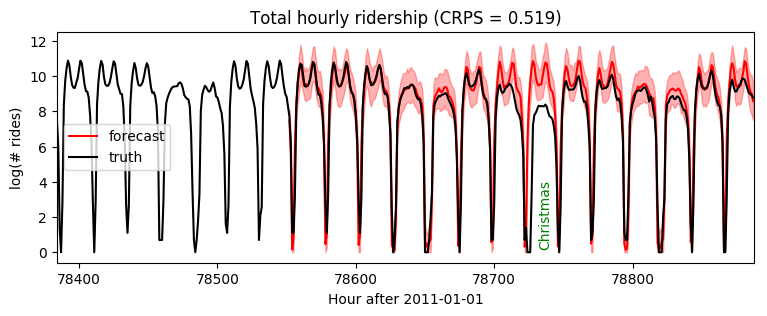
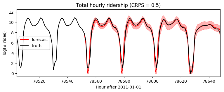
绘制未来两周的数据预测图,我们看到大部分预测是合理的,但在圣诞节出现了异常,乘客量被高估了。这是预料之中的,因为我们尚未建模年度季节性或节假日。
[8]:
samples = forecaster(data[:T1], covariates, num_samples=100)
samples.clamp_(min=0)  # apply domain knowledge: the samples must be positive
p10, p50, p90 = quantile(samples, (0.1, 0.5, 0.9)).squeeze(-1)
crps = eval_crps(samples, data[T1:])
print(samples.shape, p10.shape)

plt.figure(figsize=(9, 3))
plt.fill_between(torch.arange(T1, T2), p10, p90, color="red", alpha=0.3)
plt.plot(torch.arange(T1, T2), p50, 'r-', label='forecast')
plt.plot(torch.arange(T1 - 24 * 7, T2),
         data[T1 - 24 * 7: T2], 'k-', label='truth')
plt.title("Total hourly ridership (CRPS = {:0.3g})".format(crps))
plt.ylabel("log(# rides)")
plt.xlabel("Hour after 2011-01-01")
plt.xlim(T1 - 24 * 7, T2)
plt.text(78732, 3.5, "Christmas", rotation=90, color="green")
plt.legend(loc="best");
torch.Size([100, 336, 1]) torch.Size([336])
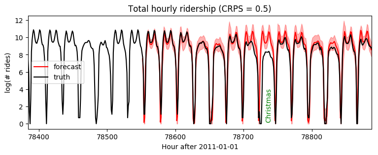
接下来,让我们将模型更改为使用异方差观测噪声,具体取决于一周中的小时数。
[9]:
class Model2(ForecastingModel):
    def model(self, zero_data, covariates):
        duration = zero_data.size(-2)
        prediction = periodic_repeat(means, duration, dim=-1).unsqueeze(-1)

        init_dist = dist.Normal(0, 10).expand([1]).to_event(1)
        timescale = pyro.sample("timescale", dist.LogNormal(math.log(24), 1))
        trans_matrix = torch.exp(-1 / timescale)[..., None, None]
        trans_scale = pyro.sample("trans_scale", dist.LogNormal(-0.5 * math.log(24), 1))
        trans_dist = dist.Normal(0, trans_scale.unsqueeze(-1)).to_event(1)
        obs_matrix = torch.tensor([[1.]])

        # To model heteroskedastic observation noise, we'll sample obs_scale inside a plate,
        # then repeat to full duration. This is the only change from Model1.
        with pyro.plate("hour_of_week", 24 * 7, dim=-1):
            obs_scale = pyro.sample("obs_scale", dist.LogNormal(-2, 1))
        obs_scale = periodic_repeat(obs_scale, duration, dim=-1)

        obs_dist = dist.Normal(0, obs_scale.unsqueeze(-1)).to_event(1)
        noise_dist = dist.GaussianHMM(
            init_dist, trans_matrix, trans_dist, obs_matrix, obs_dist, duration=duration)
        self.predict(noise_dist, prediction)
[10]:
%%time
pyro.set_rng_seed(1)
pyro.clear_param_store()
covariates = torch.zeros(len(data), 0)  # empty
forecaster = Forecaster(Model2(), data[:T1], covariates[:T1], learning_rate=0.1, num_steps=400)
for name, value in forecaster.guide.median().items():
    if value.numel() == 1:
        print("{} = {:0.4g}".format(name, value.item()))
INFO     step    0 loss = 0.954783
INFO     step  100 loss = -0.0344435
INFO     step  200 loss = -0.0373581
INFO     step  300 loss = -0.0376129
timescale = 61.41
trans_scale = 0.1082
CPU times: user 28.1 s, sys: 1.34 s, total: 29.5 s
Wall time: 29.6 s
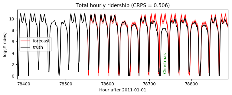
请注意,这使我们能够获得更长的时间尺度,从而实现更准确的短期预测
[11]:
samples = forecaster(data[:T1], covariates, num_samples=100)
samples.clamp_(min=0)  # apply domain knowledge: the samples must be positive
p10, p50, p90 = quantile(samples, (0.1, 0.5, 0.9)).squeeze(-1)
crps = eval_crps(samples, data[T1:])

plt.figure(figsize=(9, 3))
plt.fill_between(torch.arange(T1, T2), p10, p90, color="red", alpha=0.3)
plt.plot(torch.arange(T1, T2), p50, 'r-', label='forecast')
plt.plot(torch.arange(T1 - 24 * 7, T2),
         data[T1 - 24 * 7: T2], 'k-', label='truth')
plt.title("Total hourly ridership (CRPS = {:0.3g})".format(crps))
plt.ylabel("log(# rides)")
plt.xlabel("Hour after 2011-01-01")
plt.xlim(T1 - 24 * 7, T2)
plt.text(78732, 3.5, "Christmas", rotation=90, color="green")
plt.legend(loc="best");
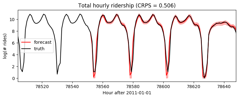
[12]:
plt.figure(figsize=(9, 3))
plt.fill_between(torch.arange(T1, T2), p10, p90, color="red", alpha=0.3)
plt.plot(torch.arange(T1, T2), p50, 'r-', label='forecast')
plt.plot(torch.arange(T1 - 24 * 7, T2),
         data[T1 - 24 * 7: T2], 'k-', label='truth')
plt.title("Total hourly ridership (CRPS = {:0.3g})".format(crps))
plt.ylabel("log(# rides)")
plt.xlabel("Hour after 2011-01-01")
plt.xlim(T1 - 24 * 2, T1 + 24 * 4)
plt.legend(loc="best");
使用 LinearHMM 进行重尾建模
接下来,让我们将模型更改为线性-Stable 动力系统,该系统在过程噪声和观测噪声中都表现出可学习的重尾行为。正如我们在单变量教程中已经看到的那样,这将需要 poutine.reparam() 对 Stable 分布进行特殊处理。对于状态空间模型,我们将 LinearHMMReparam 与其他重参数化器(如 StableReparam 和 SymmetricStableReparam)结合使用。所有重参数化器都保留生成模型的行为,仅用于通过辅助变量方法实现推断。
[13]:
class Model3(ForecastingModel):
    def model(self, zero_data, covariates):
        duration = zero_data.size(-2)
        prediction = periodic_repeat(means, duration, dim=-1).unsqueeze(-1)

        # First sample the Gaussian-like parameters as in previous models.
        init_dist = dist.Normal(0, 10).expand([1]).to_event(1)
        timescale = pyro.sample("timescale", dist.LogNormal(math.log(24), 1))
        trans_matrix = torch.exp(-1 / timescale)[..., None, None]
        trans_scale = pyro.sample("trans_scale", dist.LogNormal(-0.5 * math.log(24), 1))
        obs_matrix = torch.tensor([[1.]])
        with pyro.plate("hour_of_week", 24 * 7, dim=-1):
            obs_scale = pyro.sample("obs_scale", dist.LogNormal(-2, 1))
        obs_scale = periodic_repeat(obs_scale, duration, dim=-1)

        # In addition to the Gaussian parameters, we will learn a global stability
        # parameter to determine tail weights, and an observation skew parameter.
        stability = pyro.sample("stability", dist.Uniform(1, 2).expand([1]).to_event(1))
        skew = pyro.sample("skew", dist.Uniform(-1, 1).expand([1]).to_event(1))

        # Next we construct stable distributions and a linear-stable HMM distribution.
        trans_dist = dist.Stable(stability, 0, trans_scale.unsqueeze(-1)).to_event(1)
        obs_dist = dist.Stable(stability, skew, obs_scale.unsqueeze(-1)).to_event(1)
        noise_dist = dist.LinearHMM(
            init_dist, trans_matrix, trans_dist, obs_matrix, obs_dist, duration=duration)

        # Finally we use a reparameterizer to enable inference.
        rep = LinearHMMReparam(None,                     # init_dist is already Gaussian.
                               SymmetricStableReparam(), # trans_dist is symmetric.
                               StableReparam())          # obs_dist is asymmetric.
        with poutine.reparam(config={"residual": rep}):
            self.predict(noise_dist, prediction)
请注意,由于该模型引入了通过变分推断学习的辅助变量,梯度方差较高,我们需要训练更长时间。
[14]:
%%time
pyro.set_rng_seed(1)
pyro.clear_param_store()
covariates = torch.zeros(len(data), 0)  # empty
forecaster = Forecaster(Model3(), data[:T1], covariates[:T1], learning_rate=0.1)
for name, value in forecaster.guide.median().items():
    if value.numel() == 1:
        print("{} = {:0.4g}".format(name, value.item()))
INFO     step    0 loss = 42.9188
INFO     step  100 loss = 0.243742
INFO     step  200 loss = 0.112491
INFO     step  300 loss = 0.0320302
INFO     step  400 loss = -0.0424252
INFO     step  500 loss = -0.0763611
INFO     step  600 loss = -0.108585
INFO     step  700 loss = -0.129246
INFO     step  800 loss = -0.143037
INFO     step  900 loss = -0.173499
INFO     step 1000 loss = -0.172329
timescale = 11.29
trans_scale = 0.04193
stability = 1.68
skew = -0.0001891
CPU times: user 2min 57s, sys: 21.9 s, total: 3min 19s
Wall time: 3min 19s
[15]:
samples = forecaster(data[:T1], covariates, num_samples=100)
samples.clamp_(min=0)  # apply domain knowledge: the samples must be positive
p10, p50, p90 = quantile(samples, (0.1, 0.5, 0.9)).squeeze(-1)
crps = eval_crps(samples, data[T1:])

plt.figure(figsize=(9, 3))
plt.fill_between(torch.arange(T1, T2), p10, p90, color="red", alpha=0.3)
plt.plot(torch.arange(T1, T2), p50, 'r-', label='forecast')
plt.plot(torch.arange(T1 - 24 * 7, T2),
         data[T1 - 24 * 7: T2], 'k-', label='truth')
plt.title("Total hourly ridership (CRPS = {:0.3g})".format(crps))
plt.ylabel("log(# rides)")
plt.xlabel("Hour after 2011-01-01")
plt.xlim(T1 - 24 * 7, T2)
plt.text(78732, 3.5, "Christmas", rotation=90, color="green")
plt.legend(loc="best");
[16]:
plt.figure(figsize=(9, 3))
plt.fill_between(torch.arange(T1, T2), p10, p90, color="red", alpha=0.3)
plt.plot(torch.arange(T1, T2), p50, 'r-', label='forecast')
plt.plot(torch.arange(T1 - 24 * 7, T2),
         data[T1 - 24 * 7: T2], 'k-', label='truth')
plt.title("Total hourly ridership (CRPS = {:0.3g})".format(crps))
plt.ylabel("log(# rides)")
plt.xlabel("Hour after 2011-01-01")
plt.xlim(T1 - 24 * 2, T1 + 24 * 4)
plt.legend(loc="best");
[ ]: