预测 I: 单变量、厚尾
本教程介绍 pyro.contrib.forecast 模块,这是一个使用 Pyro 模型进行预测的框架。本教程仅涵盖单变量模型和简单似然。本教程假设读者已熟悉 SVI 和 张量形状。
另请参阅
摘要
创建预测模型
创建一个 ForecastingModel 类的子类。
使用标准 Pyro 语法实现 .model(zero_data, covariates) 方法。
在 self.time_plate 上下文内部对所有时间局部变量进行采样。
最后调用 .predict(noise_dist, prediction) 方法。
要训练预测模型,创建一个 Forecaster 对象。
训练可能会不稳定,你需要调整超参数并随机重启。
重参数化有助于学习,例如 LocScaleReparam。
要预测未来,从一个以数据和协变量为条件的
Forecaster对象中抽取样本。要对季节性建模,使用辅助函数 periodic_features(), periodic_repeat() 和 periodic_cumsum()。
要对厚尾数据建模,使用 Stable 分布和 StableReparam。
要评估结果,使用 backtest() 辅助函数或低层损失函数。
[1]:
import torch
import pyro
import pyro.distributions as dist
import pyro.poutine as poutine
from pyro.contrib.examples.bart import load_bart_od
from pyro.contrib.forecast import ForecastingModel, Forecaster, backtest, eval_crps
from pyro.infer.reparam import LocScaleReparam, StableReparam
from pyro.ops.tensor_utils import periodic_cumsum, periodic_repeat, periodic_features
from pyro.ops.stats import quantile
import matplotlib.pyplot as plt

%matplotlib inline
assert pyro.__version__.startswith('1.9.1')
pyro.set_rng_seed(20200221)
[2]:
dataset = load_bart_od()
print(dataset.keys())
print(dataset["counts"].shape)
print(" ".join(dataset["stations"]))
dict_keys(['stations', 'start_date', 'counts'])
torch.Size([78888, 50, 50])
12TH 16TH 19TH 24TH ANTC ASHB BALB BAYF BERY CAST CIVC COLM COLS CONC DALY DBRK DELN DUBL EMBR FRMT FTVL GLEN HAYW LAFY LAKE MCAR MLBR MLPT MONT NBRK NCON OAKL ORIN PCTR PHIL PITT PLZA POWL RICH ROCK SANL SBRN SFIA SHAY SSAN UCTY WARM WCRK WDUB WOAK
Pyro 预测框架简介
Pyro 的预测框架包括: - 一个 ForecastingModel 基类,其 .model() 方法可以针对自定义预测模型实现;- 一个 Forecaster 类,它使用 ForecastingModel 进行训练和预测;以及 - 一个 backtest() 辅助函数,用于评估模型在多个指标上的表现。
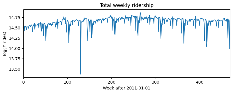
考虑一个简单的单变量数据集,例如 BART 火车 在整个网络中所有车站汇总的周载客量。这个数据大致呈对数关系,因此我们进行对数变换以进行建模。
[3]:
T, O, D = dataset["counts"].shape
data = dataset["counts"][:T // (24 * 7) * 24 * 7].reshape(T // (24 * 7), -1).sum(-1).log()
data = data.unsqueeze(-1)
plt.figure(figsize=(9, 3))
plt.plot(data)
plt.title("Total weekly ridership")
plt.ylabel("log(# rides)")
plt.xlabel("Week after 2011-01-01")
plt.xlim(0, len(data));
让我们从一个简单的对数线性回归模型开始,没有趋势或季节性。请注意,虽然此示例是单变量的,但 Pyro 的预测框架是多变量的,因此我们经常需要使用 .unsqueeze(-1)、.expand([1]) 和 .to_event(1) 进行重塑。
[4]:
# First we need some boilerplate to create a class and define a .model() method.
class Model1(ForecastingModel):
    # We then implement the .model() method. Since this is a generative model, it shouldn't
    # look at data; however it is convenient to see the shape of data we're supposed to
    # generate, so this inputs a zeros_like(data) tensor instead of the actual data.
    def model(self, zero_data, covariates):
        data_dim = zero_data.size(-1)  # Should be 1 in this univariate tutorial.
        feature_dim = covariates.size(-1)

        # The first part of the model is a probabilistic program to create a prediction.
        # We use the zero_data as a template for the shape of the prediction.
        bias = pyro.sample("bias", dist.Normal(0, 10).expand([data_dim]).to_event(1))
        weight = pyro.sample("weight", dist.Normal(0, 0.1).expand([feature_dim]).to_event(1))
        prediction = bias + (weight * covariates).sum(-1, keepdim=True)
        # The prediction should have the same shape as zero_data (duration, obs_dim),
        # but may have additional sample dimensions on the left.
        assert prediction.shape[-2:] == zero_data.shape

        # The next part of the model creates a likelihood or noise distribution.
        # Again we'll be Bayesian and write this as a probabilistic program with
        # priors over parameters.
        noise_scale = pyro.sample("noise_scale", dist.LogNormal(-5, 5).expand([1]).to_event(1))
        noise_dist = dist.Normal(0, noise_scale)

        # The final step is to call the .predict() method.
        self.predict(noise_dist, prediction)
现在我们可以通过创建一个 Forecaster 对象来训练这个模型。我们将数据分割为 [T0,T1) 用于训练,[T1,T2) 用于测试。
[5]:
T0 = 0              # begining
T2 = data.size(-2)  # end
T1 = T2 - 52        # train/test split
[6]:
%%time
pyro.set_rng_seed(1)
pyro.clear_param_store()
time = torch.arange(float(T2)) / 365
covariates = torch.stack([time], dim=-1)
forecaster = Forecaster(Model1(), data[:T1], covariates[:T1], learning_rate=0.1)
INFO     step    0 loss = 484401
INFO     step  100 loss = 0.609042
INFO     step  200 loss = -0.535144
INFO     step  300 loss = -0.605789
INFO     step  400 loss = -0.59744
INFO     step  500 loss = -0.596203
INFO     step  600 loss = -0.614217
INFO     step  700 loss = -0.612415
INFO     step  800 loss = -0.613236
INFO     step  900 loss = -0.59879
INFO     step 1000 loss = -0.601271
CPU times: user 4.37 s, sys: 30.4 ms, total: 4.4 s
Wall time: 4.4 s
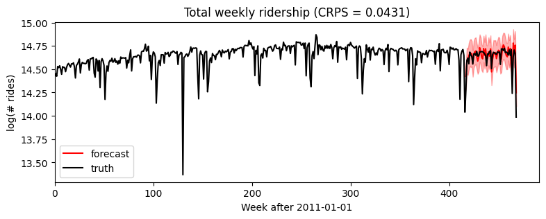
接下来我们可以通过从预测器中抽取后验样本进行评估,传入全部协变量但仅部分数据。我们将使用 Pyro 的 quantile() 函数来绘制中位数和 80% 置信区间。为了评估拟合优度,我们将使用 eval_crps() 计算 连续分级概率得分 (Continuous Ranked Probability Score);这是一个评估厚尾分布分布拟合优度的良好指标。
[7]:
samples = forecaster(data[:T1], covariates, num_samples=1000)
p10, p50, p90 = quantile(samples, (0.1, 0.5, 0.9)).squeeze(-1)
crps = eval_crps(samples, data[T1:])
print(samples.shape, p10.shape)

plt.figure(figsize=(9, 3))
plt.fill_between(torch.arange(T1, T2), p10, p90, color="red", alpha=0.3)
plt.plot(torch.arange(T1, T2), p50, 'r-', label='forecast')
plt.plot(data, 'k-', label='truth')
plt.title("Total weekly ridership (CRPS = {:0.3g})".format(crps))
plt.ylabel("log(# rides)")
plt.xlabel("Week after 2011-01-01")
plt.xlim(0, None)
plt.legend(loc="best");
torch.Size([1000, 52, 1]) torch.Size([52])
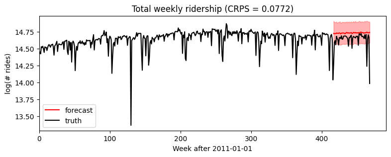
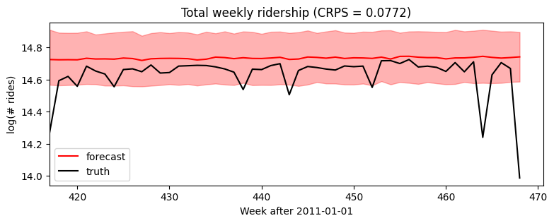
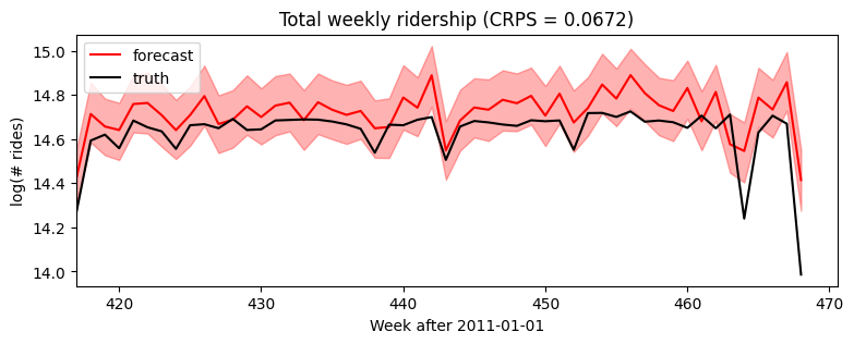
放大只看预测区域,我们发现这个模型忽略了季节性行为。
[8]:
plt.figure(figsize=(9, 3))
plt.fill_between(torch.arange(T1, T2), p10, p90, color="red", alpha=0.3)
plt.plot(torch.arange(T1, T2), p50, 'r-', label='forecast')
plt.plot(torch.arange(T1, T2), data[T1:], 'k-', label='truth')
plt.title("Total weekly ridership (CRPS = {:0.3g})".format(crps))
plt.ylabel("log(# rides)")
plt.xlabel("Week after 2011-01-01")
plt.xlim(T1, None)
plt.legend(loc="best");
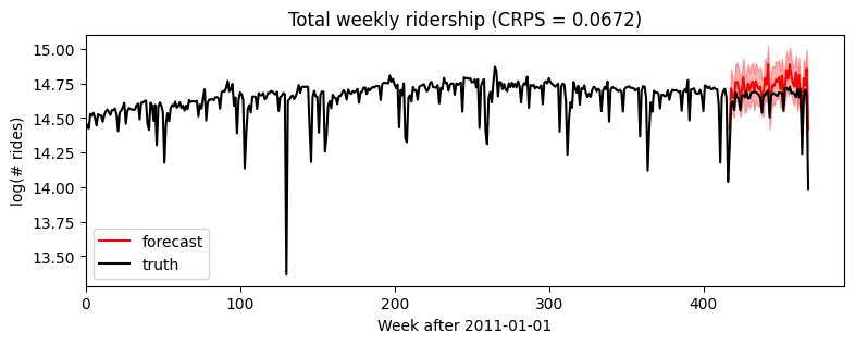
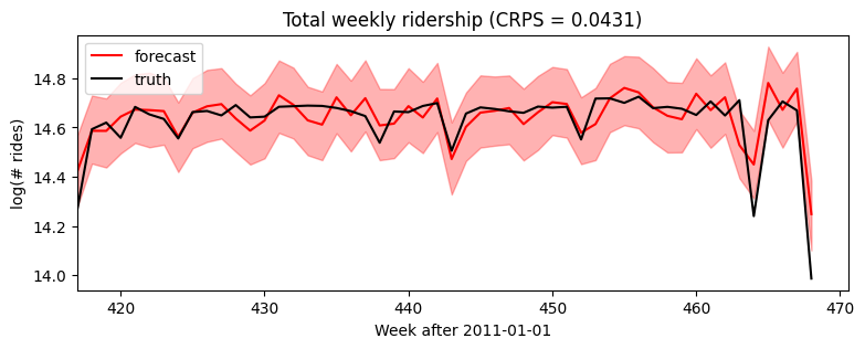
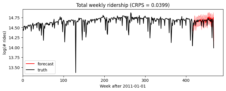
我们可以简单地添加新的协变量来增加一个年度季节性分量(请注意,我们已经在模型中处理了 feature_dim > 1 的情况)。
[9]:
%%time
pyro.set_rng_seed(1)
pyro.clear_param_store()
time = torch.arange(float(T2)) / 365
covariates = torch.cat([time.unsqueeze(-1),
                        periodic_features(T2, 365.25 / 7)], dim=-1)
forecaster = Forecaster(Model1(), data[:T1], covariates[:T1], learning_rate=0.1)
INFO     step    0 loss = 53174.4
INFO     step  100 loss = 0.519148
INFO     step  200 loss = -0.0264822
INFO     step  300 loss = -0.314983
INFO     step  400 loss = -0.413243
INFO     step  500 loss = -0.487756
INFO     step  600 loss = -0.472516
INFO     step  700 loss = -0.595866
INFO     step  800 loss = -0.500985
INFO     step  900 loss = -0.558623
INFO     step 1000 loss = -0.589603
CPU times: user 4.5 s, sys: 34.3 ms, total: 4.53 s
Wall time: 4.54 s
[10]:
samples = forecaster(data[:T1], covariates, num_samples=1000)
p10, p50, p90 = quantile(samples, (0.1, 0.5, 0.9)).squeeze(-1)
crps = eval_crps(samples, data[T1:])

plt.figure(figsize=(9, 3))
plt.fill_between(torch.arange(T1, T2), p10, p90, color="red", alpha=0.3)
plt.plot(torch.arange(T1, T2), p50, 'r-', label='forecast')
plt.plot(data, 'k-', label='truth')
plt.title("Total weekly ridership (CRPS = {:0.3g})".format(crps))
plt.ylabel("log(# rides)")
plt.xlabel("Week after 2011-01-01")
plt.xlim(0, None)
plt.legend(loc="best");
[11]:
plt.figure(figsize=(9, 3))
plt.fill_between(torch.arange(T1, T2), p10, p90, color="red", alpha=0.3)
plt.plot(torch.arange(T1, T2), p50, 'r-', label='forecast')
plt.plot(torch.arange(T1, T2), data[T1:], 'k-', label='truth')
plt.title("Total weekly ridership (CRPS = {:0.3g})".format(crps))
plt.ylabel("log(# rides)")
plt.xlabel("Week after 2011-01-01")
plt.xlim(T1, None)
plt.legend(loc="best");
时间局部随机变量: self.time_plate
到目前为止,我们已经看到了 ForecastingModel.model() 方法和 self.predict()。预测特有的最后一部分语法是用于时间局部变量的 self.time_plate 上下文。为了了解其工作原理,考虑将上面我们的全局线性趋势模型更改为局部水平模型。请注意,poutine.reparam() 处理器是一个通用的 Pyro 推断技巧,并非预测特有。
[12]:
class Model2(ForecastingModel):
    def model(self, zero_data, covariates):
        data_dim = zero_data.size(-1)
        feature_dim = covariates.size(-1)
        bias = pyro.sample("bias", dist.Normal(0, 10).expand([data_dim]).to_event(1))
        weight = pyro.sample("weight", dist.Normal(0, 0.1).expand([feature_dim]).to_event(1))

        # We'll sample a time-global scale parameter outside the time plate,
        # then time-local iid noise inside the time plate.
        drift_scale = pyro.sample("drift_scale",
                                  dist.LogNormal(-20, 5).expand([1]).to_event(1))
        with self.time_plate:
            # We'll use a reparameterizer to improve variational fit. The model would still be
            # correct if you removed this context manager, but the fit appears to be worse.
            with poutine.reparam(config={"drift": LocScaleReparam()}):
                drift = pyro.sample("drift", dist.Normal(zero_data, drift_scale).to_event(1))

        # After we sample the iid "drift" noise we can combine it in any time-dependent way.
        # It is important to keep everything inside the plate independent and apply dependent
        # transforms outside the plate.
        motion = drift.cumsum(-2)  # A Brownian motion.

        # The prediction now includes three terms.
        prediction = motion + bias + (weight * covariates).sum(-1, keepdim=True)
        assert prediction.shape[-2:] == zero_data.shape

        # Construct the noise distribution and predict.
        noise_scale = pyro.sample("noise_scale", dist.LogNormal(-5, 5).expand([1]).to_event(1))
        noise_dist = dist.Normal(0, noise_scale)
        self.predict(noise_dist, prediction)
[13]:
%%time
pyro.set_rng_seed(1)
pyro.clear_param_store()
time = torch.arange(float(T2)) / 365
covariates = periodic_features(T2, 365.25 / 7)
forecaster = Forecaster(Model2(), data[:T1], covariates[:T1], learning_rate=0.1,
                        time_reparam="dct",
                       )
INFO     step    0 loss = 1.73259e+09
INFO     step  100 loss = 0.935019
INFO     step  200 loss = -0.0290582
INFO     step  300 loss = -0.193718
INFO     step  400 loss = -0.292689
INFO     step  500 loss = -0.411964
INFO     step  600 loss = -0.291355
INFO     step  700 loss = -0.414344
INFO     step  800 loss = -0.472016
INFO     step  900 loss = -0.480997
INFO     step 1000 loss = -0.540629
CPU times: user 9.47 s, sys: 56.4 ms, total: 9.52 s
Wall time: 9.54 s
[14]:
samples = forecaster(data[:T1], covariates, num_samples=1000)
p10, p50, p90 = quantile(samples, (0.1, 0.5, 0.9)).squeeze(-1)
crps = eval_crps(samples, data[T1:])

plt.figure(figsize=(9, 3))
plt.fill_between(torch.arange(T1, T2), p10, p90, color="red", alpha=0.3)
plt.plot(torch.arange(T1, T2), p50, 'r-', label='forecast')
plt.plot(data, 'k-', label='truth')
plt.title("Total weekly ridership (CRPS = {:0.3g})".format(crps))
plt.ylabel("log(# rides)")
plt.xlabel("Week after 2011-01-01")
plt.xlim(0, None)
plt.legend(loc="best");
[15]:
plt.figure(figsize=(9, 3))
plt.fill_between(torch.arange(T1, T2), p10, p90, color="red", alpha=0.3)
plt.plot(torch.arange(T1, T2), p50, 'r-', label='forecast')
plt.plot(torch.arange(T1, T2), data[T1:], 'k-', label='truth')
plt.title("Total weekly ridership (CRPS = {:0.3g})".format(crps))
plt.ylabel("log(# rides)")
plt.xlabel("Week after 2011-01-01")
plt.xlim(T1, None)
plt.legend(loc="best");
厚尾噪声
我们的最后一个单变量模型将从高斯噪声泛化到厚尾 Stable 噪声。唯一的区别是 noise_dist,它现在接受两个新参数:stability 决定尾部权重,skew 决定正向峰值与负向峰值的相对大小。
Stable 分布是正态分布的自然厚尾泛化,但由于其难以处理的密度函数,与之合作十分困难。Pyro 实现了处理 Stable 分布的辅助变量方法。为了告知 Pyro 使用这些辅助变量方法,我们将最后一行包装在 poutine.reparam() 效果处理器中,该处理器将 StableReparam 变换应用于命名为“residual”的隐式观测点。你可以通过指定 config={"my_site_name": StableReparam()} 将 Stable 分布用于其他观测点。
[16]:
class Model3(ForecastingModel):
    def model(self, zero_data, covariates):
        data_dim = zero_data.size(-1)
        feature_dim = covariates.size(-1)
        bias = pyro.sample("bias", dist.Normal(0, 10).expand([data_dim]).to_event(1))
        weight = pyro.sample("weight", dist.Normal(0, 0.1).expand([feature_dim]).to_event(1))

        drift_scale = pyro.sample("drift_scale", dist.LogNormal(-20, 5).expand([1]).to_event(1))
        with self.time_plate:
            with poutine.reparam(config={"drift": LocScaleReparam()}):
                drift = pyro.sample("drift", dist.Normal(zero_data, drift_scale).to_event(1))
        motion = drift.cumsum(-2)  # A Brownian motion.

        prediction = motion + bias + (weight * covariates).sum(-1, keepdim=True)
        assert prediction.shape[-2:] == zero_data.shape

        # The next part of the model creates a likelihood or noise distribution.
        # Again we'll be Bayesian and write this as a probabilistic program with
        # priors over parameters.
        stability = pyro.sample("noise_stability", dist.Uniform(1, 2).expand([1]).to_event(1))
        skew = pyro.sample("noise_skew", dist.Uniform(-1, 1).expand([1]).to_event(1))
        scale = pyro.sample("noise_scale", dist.LogNormal(-5, 5).expand([1]).to_event(1))
        noise_dist = dist.Stable(stability, skew, scale)

        # We need to use a reparameterizer to handle the Stable distribution.
        # Note "residual" is the name of Pyro's internal sample site in self.predict().
        with poutine.reparam(config={"residual": StableReparam()}):
            self.predict(noise_dist, prediction)
[17]:
%%time
pyro.set_rng_seed(2)
pyro.clear_param_store()
time = torch.arange(float(T2)) / 365
covariates = periodic_features(T2, 365.25 / 7)
forecaster = Forecaster(Model3(), data[:T1], covariates[:T1], learning_rate=0.1,
                        time_reparam="dct")
for name, value in forecaster.guide.median().items():
    if value.numel() == 1:
        print("{} = {:0.4g}".format(name, value.item()))
INFO     step    0 loss = 5.92061e+07
INFO     step  100 loss = 13.6553
INFO     step  200 loss = 3.18891
INFO     step  300 loss = 0.884046
INFO     step  400 loss = 0.27383
INFO     step  500 loss = -0.0354842
INFO     step  600 loss = -0.211247
INFO     step  700 loss = -0.311198
INFO     step  800 loss = -0.259799
INFO     step  900 loss = -0.326406
INFO     step 1000 loss = -0.306335
bias = 14.64
drift_scale = 3.234e-08
noise_stability = 1.937
noise_skew = 0.004095
noise_scale = 0.06038
CPU times: user 19.5 s, sys: 103 ms, total: 19.6 s
Wall time: 19.7 s
[18]:
samples = forecaster(data[:T1], covariates, num_samples=1000)
p10, p50, p90 = quantile(samples, (0.1, 0.5, 0.9)).squeeze(-1)
crps = eval_crps(samples, data[T1:])

plt.figure(figsize=(9, 3))
plt.fill_between(torch.arange(T1, T2), p10, p90, color="red", alpha=0.3)
plt.plot(torch.arange(T1, T2), p50, 'r-', label='forecast')
plt.plot(data, 'k-', label='truth')
plt.title("Total weekly ridership (CRPS = {:0.3g})".format(crps))
plt.ylabel("log(# rides)")
plt.xlabel("Week after 2011-01-01")
plt.xlim(0, None)
plt.legend(loc="best");
[19]:
plt.figure(figsize=(9, 3))
plt.fill_between(torch.arange(T1, T2), p10, p90, color="red", alpha=0.3)
plt.plot(torch.arange(T1, T2), p50, 'r-', label='forecast')
plt.plot(torch.arange(T1, T2), data[T1:], 'k-', label='truth')
plt.title("Total weekly ridership (CRPS = {:0.3g})".format(crps))
plt.ylabel("log(# rides)")
plt.xlabel("Week after 2011-01-01")
plt.xlim(T1, None)
plt.legend(loc="best");
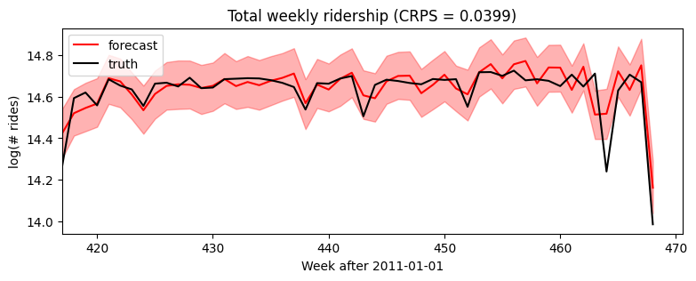
回测
为了比较我们的高斯 Model2 和 Stable Model3,我们将使用一个简单的 backtesting() 辅助函数。这个辅助函数默认评估三个指标:CRPS 评估厚尾数据的分布准确性,MAE 评估厚尾数据的点准确性,以及 RMSE 评估正态尾部数据的准确性。这里的一个微妙之处是设置 warm_start=True 以减少随机重启的需求。
[20]:
%%time
pyro.set_rng_seed(1)
pyro.clear_param_store()
windows2 = backtest(data, covariates, Model2,
                    min_train_window=104, test_window=52, stride=26,
                    forecaster_options={"learning_rate": 0.1, "time_reparam": "dct",
                                        "log_every": 1000, "warm_start": True})
INFO     Training on window [0:104], testing on window [104:156]
INFO     step    0 loss = 3543.21
INFO     step 1000 loss = 0.140962
INFO     Training on window [0:130], testing on window [130:182]
INFO     step    0 loss = 0.27281
INFO     step 1000 loss = -0.227765
INFO     Training on window [0:156], testing on window [156:208]
INFO     step    0 loss = 0.622017
INFO     step 1000 loss = -0.0232647
INFO     Training on window [0:182], testing on window [182:234]
INFO     step    0 loss = 0.181045
INFO     step 1000 loss = -0.104492
INFO     Training on window [0:208], testing on window [208:260]
INFO     step    0 loss = 0.160061
INFO     step 1000 loss = -0.184363
INFO     Training on window [0:234], testing on window [234:286]
INFO     step    0 loss = 0.0414903
INFO     step 1000 loss = -0.207943
INFO     Training on window [0:260], testing on window [260:312]
INFO     step    0 loss = -0.00223408
INFO     step 1000 loss = -0.256718
INFO     Training on window [0:286], testing on window [286:338]
INFO     step    0 loss = -0.0552213
INFO     step 1000 loss = -0.277793
INFO     Training on window [0:312], testing on window [312:364]
INFO     step    0 loss = -0.141342
INFO     step 1000 loss = -0.36945
INFO     Training on window [0:338], testing on window [338:390]
INFO     step    0 loss = -0.148779
INFO     step 1000 loss = -0.332914
INFO     Training on window [0:364], testing on window [364:416]
INFO     step    0 loss = -0.27899
INFO     step 1000 loss = -0.462222
INFO     Training on window [0:390], testing on window [390:442]
INFO     step    0 loss = -0.328539
INFO     step 1000 loss = -0.463518
INFO     Training on window [0:416], testing on window [416:468]
INFO     step    0 loss = -0.400719
INFO     step 1000 loss = -0.494253
CPU times: user 1min 57s, sys: 502 ms, total: 1min 57s
Wall time: 1min 57s
[21]:
%%time
pyro.set_rng_seed(1)
pyro.clear_param_store()
windows3 = backtest(data, covariates, Model3,
                    min_train_window=104, test_window=52, stride=26,
                    forecaster_options={"learning_rate": 0.1, "time_reparam": "dct",
                                        "log_every": 1000, "warm_start": True})
INFO     Training on window [0:104], testing on window [104:156]
INFO     step    0 loss = 1852.88
INFO     step 1000 loss = 0.533988
INFO     Training on window [0:130], testing on window [130:182]
INFO     step    0 loss = 2.60906
INFO     step 1000 loss = 0.0715323
INFO     Training on window [0:156], testing on window [156:208]
INFO     step    0 loss = 2.60063
INFO     step 1000 loss = 0.110426
INFO     Training on window [0:182], testing on window [182:234]
INFO     step    0 loss = 1.99784
INFO     step 1000 loss = 0.020393
INFO     Training on window [0:208], testing on window [208:260]
INFO     step    0 loss = 1.63004
INFO     step 1000 loss = -0.0936131
INFO     Training on window [0:234], testing on window [234:286]
INFO     step    0 loss = 1.33227
INFO     step 1000 loss = -0.114948
INFO     Training on window [0:260], testing on window [260:312]
INFO     step    0 loss = 1.19163
INFO     step 1000 loss = -0.193086
INFO     Training on window [0:286], testing on window [286:338]
INFO     step    0 loss = 1.01131
INFO     step 1000 loss = -0.242592
INFO     Training on window [0:312], testing on window [312:364]
INFO     step    0 loss = 0.983859
INFO     step 1000 loss = -0.279851
INFO     Training on window [0:338], testing on window [338:390]
INFO     step    0 loss = 0.560554
INFO     step 1000 loss = -0.209488
INFO     Training on window [0:364], testing on window [364:416]
INFO     step    0 loss = 0.716816
INFO     step 1000 loss = -0.369162
INFO     Training on window [0:390], testing on window [390:442]
INFO     step    0 loss = 0.391474
INFO     step 1000 loss = -0.45527
INFO     Training on window [0:416], testing on window [416:468]
INFO     step    0 loss = 0.37326
INFO     step 1000 loss = -0.508014
CPU times: user 4min 1s, sys: 960 ms, total: 4min 2s
Wall time: 4min 2s
[22]:
fig, axes = plt.subplots(3, figsize=(8, 6), sharex=True)
axes[0].set_title("Gaussian versus Stable accuracy over {} windows".format(len(windows2)))
axes[0].plot([w["crps"] for w in windows2], "b<", label="Gaussian")
axes[0].plot([w["crps"] for w in windows3], "r>", label="Stable")
axes[0].set_ylabel("CRPS")
axes[1].plot([w["mae"] for w in windows2], "b<", label="Gaussian")
axes[1].plot([w["mae"] for w in windows3], "r>", label="Stable")
axes[1].set_ylabel("MAE")
axes[2].plot([w["rmse"] for w in windows2], "b<", label="Gaussian")
axes[2].plot([w["rmse"] for w in windows3], "r>", label="Stable")
axes[2].set_ylabel("RMSE")
axes[0].legend(loc="best")
plt.tight_layout()
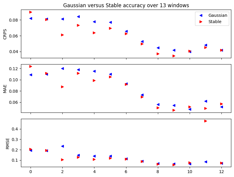
请注意,RMSE 是评估厚尾数据的差劲指标。我们的 Stable 模型尾部非常厚,其方差是无穷大,因此我们不能期望 RMSE 收敛,因此会出现偶尔的离群点。
[ ]: